 Skip to content


Bayesian methods have become increasingly popular over the last few years underpinned by the continuing development of intensive computer methodologies (particularly Markov chain Monte Carlo (MCMC)) and enabled by computer capabilities making them more practical to use. But how do they compare to classical (‘Frequentist’) statistics?
Evaluating traditional approaches: Bayesian vs. Frequentist
Most statistical analyses focus on three things:
- summaries or parameter estimates, which are often treatment means in classical statistics;
- measures of uncertainty of the estimates, such as standard error, Least Significant Difference, or a 95% confidence intervals; and
- ‘tests’, which give p-values, often comparing the mean for one treatment with another.
There are several problems with this approach, including:
(i) An assumption that you have no prior information about the likely size of the ‘true’ means when prior information is often available.
(ii) Confidence intervals (e.g. 95%) are interpreted as ‘there is a 95% chance that the ‘true’ mean lies in the interval’, but actually mean ‘if a
very large number of exact repeats of a trial are carried out, 95% of the confidence limits will contain the ‘true’ mean’ – hard to digest!
(iii) p-values are widely interpreted to indicate that two treatment means are ‘different’ (usually, p-value<0.05)[1].
[1] Many references show this. See e.g. https://vsni.co.uk/blogs/never-accept-the-null-hypothesis
However, a p-value actually means: The probability of getting the observed test statistic or one more extreme
GIVEN THAT
the null hypothesis of ‘no difference’ is true.
To show that two means are different, what we really want is the reverse of this: The probability that the null hypothesis of ‘no difference’ is true given the data collected. p-values do not give us this.
The Bayes’ equation: unlocking conditional probabilities
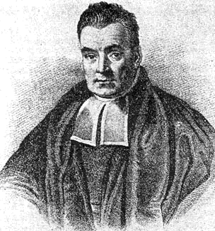
Bayes developed an equation that allows us to ‘reverse’ conditional probabilities, converting the probability of A given B into the probability of B give A, which is close to what we want to do. Bayes’ equation does this using an association with the probability of A and B both occurring:

Where P() is the probability of event A, or B; ‘|’ means ‘given’, and P(A⋂B) is the probability of both A and B occurring.
This equation can be manipulated algebraically to remove the need to know P(B), by replacing P(B) with the integral (for continuous data) or sum (discreate data like for counts) of P(A) x P(B│A) over all possible values of A:

In Bayesian analysis, A is a parameter or parameters we wish to estimate, and B is a set of data we have collected. Bayes’ theorem allows our prior ‘beliefs’ P(A) about the value of A to be updated by information from collected data B in terms of the likelihood P(B|A), to give a posterior distribution P(A|B). Thus, if A is the Null Hypothesis of ‘no difference’ between treatment means, Bayes’ equation can be used to get the probability of this null hypothesis being true given the data B, using our prior belief about the Null hypothesis and the likelihood for a data B set given that A is true. Mathematically, this equation is always true: the controversies associated with using Bayes’ equation are not associated with the equation itself.
Whilst P(A), P(B/A) and P(B) can be single values, it is more usual for them to be probability distributions. In most cases, the calculation of P(A|B) can be very difficult or impossible. Various methods have been developed to get around this problem, the most common being the MCMC methods.
Bayesian vs. Frequentist interpretation: a nuanced comparison
For (i) above, prior beliefs can be included in the analysis.
For (ii) above, the posterior distribution is generally summarised as the mean with 95% ‘credible intervals’. There is a 95% chance of the ‘true’ mean value being in the interval.
Finally, for (iii) above, any ‘tests’ are based on what we want: the probability of a hypothesis being true given the collected data.
A further advantage of Bayesian methods is that they can be used for models where there is no available ‘standard’ method.
So why doesn’t everyone use Bayesian methods?
First, it can be extremely time-consuming and computer-resource hungry to fit a Bayesian model. This is primarily because MCMC is a sampling method and requires a few thousand iterations. Second, specifying the model can be difficult depending on the software used. Developments in software have made model specification easier, and modern computers and sophisticated algorithms speed up the model fitting, but Bayesian methods are still more challenging to use than classical methods.
Third, there is often no prior information, and Bayesian methods require a prior. So called ‘uninformative’ priors have been developed to address this. However, there is much controversy associated with the choice and use of uninformative priors. With uninformative priors, Bayesian estimates and credible intervals are often very similar to classical estimates and confidence intervals, and thus it can be hard to justify the extra effort and expense involved.
Finally, there is no consensus on the equivalent to the ‘significance’ test. For a simple test such as the difference between two treatments, the Bayesian equivalent is to see whether the 95% credible interval for the posterior distribution of the difference contains 0 (whence, ‘no difference’). There are also statistics such as the Deviance Information Criterion (DIC) and Bayes Factor (BF): these allow two different models to be compared, but there is no consensus on how to interpret these, and they are generally not easily available within Bayes’ software.
A practical example: ANOVA vs. Bayesian analysis
Five replicates of eight potato cultivars (Cv), were laid out in randomised blocks, four plants per plot. Two plants/plot were inoculated with a potato virus; two not inoculated. The mean weight over individual tubers per plant was analysed. This is therefore a split-plot design, with cultivar the main plot treatment and inoculation the split plot treatment, with four ‘split plots’ (plants) per plot.
Analysis of variance in Genstat:
Four commands were required in Genstat to specify the model, do the analysis, and produce model checking plots, which took < 0.5 seconds to fit.
The ANOVA table looks like this:

Inoculation had little effect on tuber weight, but there was variability between the Cultivars. Notably, Cv1 had the lowest weight and Cv7 the highest.

Means and estimated 95% confidence intervals from ANOVA
WinBugs Bayesian analysis
The model fitted was the same as for ANOVA, with uninformative normal priors for effects (mean=0, large variance). Each sub-model was then fitted, which required many lines of code per model. The full model took 20 seconds, and each subsequent model took around 10 seconds, with a total time of about a minute. This is 120 times as long as for ANOVA in Genstat. Other newer Bayesian software may fit this model more quickly, but none are likely to match ANOVA for speed.
DIC for each model:

* approx. number of parameters, including block and plot effects
The model with just Cv has the smallest DIC (-507.680). The model without an interaction but with both factors had the second lowest DIC. Thus, the primary conclusions match those from the ANOVA.

Comparisons of means and estimated 95% confidence intervals from ANOVA with estimated means and 95% credible intervals from WinBugs Bayesian analysis.


