The G×E interaction phenomenon

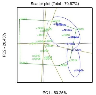
What is GxE interaction?

The genotype by environment (G×E) interaction phenomenon results from different genotypes responding to environmental variation in different ways. That is, the G×E interaction occurs when the performance of a set of genotypes depends on the environment. Whereas some genotypes may perform well across a wide range of environmental conditions (i.e., they are broadly adapted genotypes), others may perform well in only a subset of environments (i.e., they are specifically adapted genotypes). 

Breeders investigate the G×E interaction to identify genotypes well suited for use in many environments, as well as those with exceptional performance in specific environments (i.e., are well suited for use under certain environmental conditions).

Patterns of G×E interaction

To illustrate the G×E interaction, let’s consider the phenotypic response of two genotypes across two environments. The four possible patterns of phenotypic response are shown below:

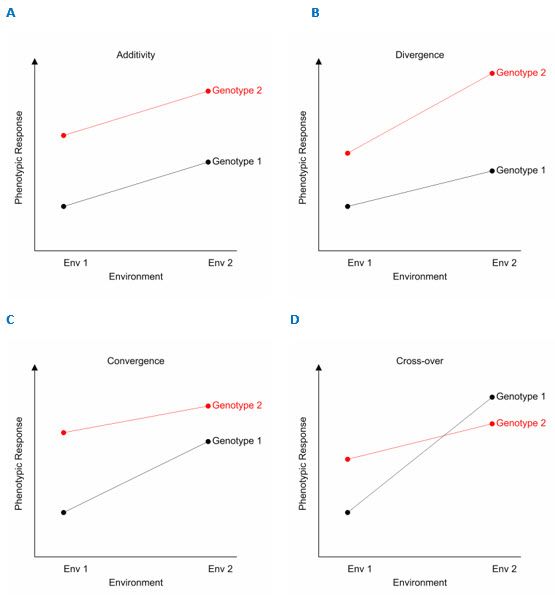
The first pattern (A) is of no interaction, where the effects of genotype and environment are independent of one another (i.e., behave additively). That is, the difference in phenotypic response between the two genotypes is the same across the two environments. In this case, Genotype 2 has a higher phenotypic response than Genotype 1 by a constant amount in both environments. The three remaining patterns (B, C, D) are non-additive. Here, the difference between genotypes changes between environments, i.e., the phenotypic performance of the genotypes is dependent on environment. The cross-over interaction (D) is arguably the most critical for breeders. It implies that the choice of the best genotype is determined by the environment, seriously hampering efforts to select genotypes that perform well across a range of environmental conditions. When the ordering of environments has a biological interpretation (e.g., ordered by say longitude, temperature or rainfall) the divergence (B) or convergence (D) patterns are perhaps more common.

The significance of type B genetic correlation

In the above figure, we have considered the effect of the G×E interaction on changes in mean phenotypic response. However, the G×E interaction can also have a consequence on the correlation between the phenotypic response of a given genotype in different environments. This is known as the Type B genetic correlation. For example, when the G×E interaction is large, the phenotypic performance of a genotype in one environment may not be very informative about its performance in another, possibly very different, environment. This results in a low Type B genetic correlation. Only those environments with similar characteristics lead to a strong positive Type B genetic correlation. Furthermore, the G×E interaction can have other effects, such as inducing heterogeneity of genetic variance across environments, where the magnitude of genetic variance is different between environments.  Let’s look at two examples that illustrate potential effects of the G×E interaction on genetic variance and correlation between two environments.

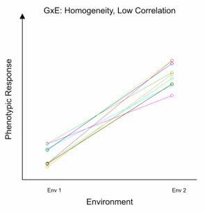
In this first example, the variation between genotypes is similar in both environments (i.e., the genetic variance is homogeneous). However, as there is no consistent pattern in relative genotypic performance between the two environments, the Type B genetic correlation is low.

Implications of genetic variance heterogeneity

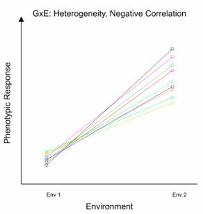
In the second example, the Type B correlation between the two environments is negative, as the cross-over means that genotypes high in Env 1 will be low in Env 2. It is also clear that the variation between genotypes in Env 1 is substantially smaller than Env 2 - this is genetic variance heterogeneity. 

Statistical tools for analyzing G×E interaction

Linear mixed models are often employed, very successfully, to quantify and describe the G×E interaction. For example, a linear mixed model with a multiplicative factor analytic (FA) model for the G×E interaction effects is generally used by plant breeders when analysing multi-environment trial (MET) data. Also very helpful for understanding the nature of the G×E interaction are AMMI and GGE biplots. These descriptive, visualisation tools enable the relationships between genotypes and environments to be explored. 

Predicting the performance of novel genotypes in different environments is essential for developing new cultivars (or breeds, in the case of animal breeding) with superior economically important traits (such as yield) and resilience to environmental stresses (such as drought). Understanding the nature of the G×E interaction helps us to do this!

Check out our other blogs related to this topic…

• Predicting the Performance of Genotypes by Multi-Environment Trial Analyses
• Using genetic correlations to improve the University of Florida's strawberry breeding program
• Which-won-where? GGE biplots in Genstat

About the author

Dr Vanessa Cave is an applied statistician interested in the application of statistics to the biosciences, in particular agriculture and ecology, and is a developer of the Genstat statistical software package. She has over 15 years of experience collaborating with scientists, using statistics to solve real-world problems.  Vanessa provides expertise on experiment and survey design, data collection and management, statistical analysis, and the interpretation of statistical findings. Her interests include statistical consultancy, mixed models, multivariate methods, statistical ecology, statistical graphics and data visualisation, and the statistical challenges related to digital agriculture.

Vanessa is currently President of the Australasian Region of the International Biometric Society, past-President of the New Zealand Statistical Association, an Associate Editor for the Agronomy Journal, on the Editorial Board of The New Zealand Veterinary Journal and an honorary academic at the University of Auckland. She has a PhD in statistics from the University of St Andrew.