Unlocking insights: analyzing field experiment data with linear mixed models in a balanced lattice square design

This blog illustrates how to analyze data from a field experiment with a balanced lattice square design using linear mixed models. We’ll consider two models: the balanced lattice square model and a spatial model.

The example data are from a field experiment conducted at Slate Hall Farm, UK, in 1976 (Gilmour et al., 1995). The experiment was set up to compare the performance of 25 varieties of barley and was designed as a balanced lattice square with six replicates laid out in a 10 x 15 rectangular grid. Each replicate contained exactly one plot for every variety. The variety grown in each plot, and the coding of the replicates and lattice blocks, is shown in the field layout below:

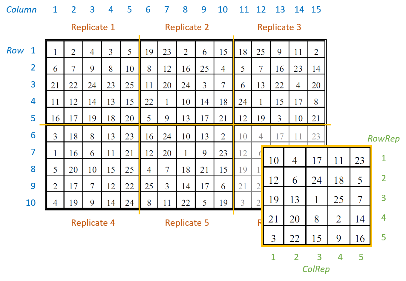
There are seven columns in the data frame: five blocking factors (Rep, RowRep, ColRep, Row, Column), one treatment factor, Variety, and the response variate, yield.

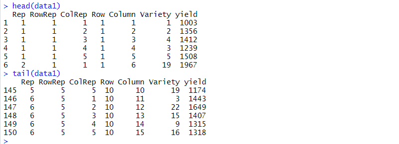
The six replicates are numbered from 1 to 6 (Rep). The lattice block numbering is coded within replicates. That is, within each replicates the lattice rows (RowRep) and lattice columns (ColRep) are both numbered from 1 to 5. The Rowand Column factors define the row and column positions within the field (rather than within each replicate).

Analysis of a balanced lattice square design

To analyze the response variable, yield, we need to identify the two basic components of the experiment: the treatment structure and the blocking (or design) structure. The treatment structure consists of the set of treatments, or treatment combinations, selected to study or to compare. In our example, there is one treatment factor with 25 levels, Variety (i.e. the 25 different varieties of barley). The blocking structure of replicates (Rep), lattice rows within replicates (Rep:RowRep), and lattice columns within replicates (Rep:ColRep) reflects the balanced lattice square design. In a mixed model analysis, the treatment factors are (usually) fitted as fixed effects and the blocking factors as random.

The balanced lattice square model is fitted in ASReml-R4 using the following code:

>; lattice.asr <;- asreml(fixed = yield ~ Variety,
random = ~ Rep + Rep:RowRep + Rep:ColRep,
data=data1)

The REML log-likelihood is -707.786.

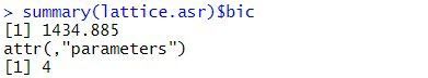
The model’s BIC is:

The estimated variance components are:

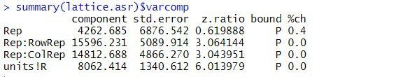
The table above contains the estimated variance components for all terms in the random model. The variance component measures the inherent variability of the term, over and above the variability of the sub-units of which it is composed. The variance components for Rep, Rep:RowRep and Rep:ColRep are estimated as 4263, 15596, and 14813, respectively. As is typical, the largest unit (replicate) is more variable than its sub-units (lattice rows and columns within replicates). The "_units!R_" component is the residual variance.

By default, fixed effects in ASReml-R4 are tested using sequential Wald tests:

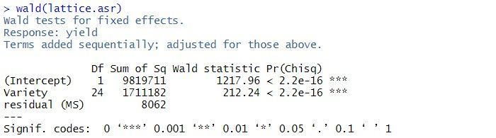
In this example, there are two terms in the summary table: the overall mean, (Intercept), and Variety. As the tests are sequential, the effect of the Variety is assessed by calculating the change in sums of squares between the two models (Intercept)+Varietyand (Intercept). The p-value (Pr(Chisq)) of  < 2.2 x 10-16 indicates that Variety is a highly significant.

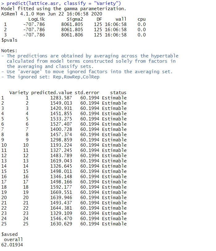
The predicted means for the Variety can be obtained using the predict() function. The standard error of the difference between any pair of variety means is 62. Note: all variety means have the same standard error as the design is balanced.

Note: the same analysis is obtained when the random model is redefined as replicates (Rep), rows within replicates (Rep_:_Row) and columns within replicates (Rep:Column).

Spatial analysis of a field experiment

As the plots are laid out in a grid, the data can also be analyzed using a spatial model. We’ll illustrate spatial analysis by fitting a model with a separable first order autoregressive process in the field row (Row) and field column (Column) directions. This is often a useful model to start the spatial modeling process.

The separable first order autoregressive spatial model is fitted in ASReml-R4 using the following code:

>; spatial.asr <;- asreml(fixed = yield ~ Variety,
residual = ~ar1(Row):ar1(Column),
data = data1)

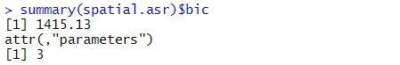
The BIC for this spatial model is:

The estimated variance components and sequential Wald tests are:

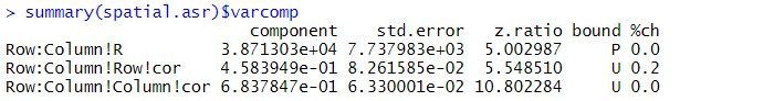
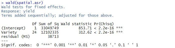
The residual variance is 38713, the estimated row correlation is 0.458, and the estimated column correlation is 0.684. As for the balanced lattice square model, there is strong evidence of a Variety effect (p-value < 2.2 x 10-16).

A log-likelihood ratio test cannot be used to compare the balanced lattice square model with the spatial models, as the variance models are not nested. However, the two models can be compared using BIC. As the spatial model has a smaller BIC (1415) than the balanced lattice square model (1435), of the two models explored in this blog, it is chosen as the preferred model. However, selecting the optimal spatial model can be difficult. The current spatial model can be extended by including measurement error (or nugget effect) or revised by selecting a different variance model for the spatial effects.

References

Butler, D.G., Cullis, B.R., Gilmour, A. R., Gogel, B.G. and Thompson, R. (2017). ASReml-R Reference Manual Version 4. VSN International Ltd, Hemel Hempstead, HP2 4TP UK.

Gilmour, A.R., Thompson, R. & Cullis, B.R. (1995). Average Information REML, an efficient algorithm for variance parameter estimation in linear mixed models. Biometrics, 51, 1440-1450.