Meta analysis using linear mixed models

What is meta-analysis?

Meta-analysis is a statistical tool that allows us to combine information from related, but independent studies, that all have as an objective to estimate or compare the same effects from contrasting treatments. Meta-analysis is widely used in many research areas where an extensive literature review is performed to identify studies that had a similar research question. These are later combined using meta-analysis to estimate a single combined effect. Meta-analyses are commonly used to answer healthcare and medical questions, where they are widely accepted, but they also are used in many other scientific fields.

By combining several sources of information, meta-analyses have the advantage of greater statistical power, therefore increasing our chance of detecting a significant difference. They also allow us to assess the variability between studies, and help us to understand potential differences between the outcomes of the original studies.

The underlying premise in meta-analysis is that we are collecting information from a group of, say n, studies that individually estimated a parameter of interest, say . It is reasonable to consider that this parameter has some statistical properties. Mainly we assume that it belongs to a Normal distribution with unknown mean and variance. Hence, mathematically we say:

In meta-analysis, the target population parameter θ can correspond to any of several statistics, such as a treatment mean, a difference between treatments; or more commonly in clinical trials, the log-odds ratio or relative risk.

Understanding the fixed-effect model

There are two models that are commonly used to perform meta-analyses: the fixed-effect model and the random-effects model. For the fixed-effect model, it is assumed that there is only a single unique true effect our single θ above, which is estimated from a random sample of studies. That is, the fixed-effect model assumes that there is a single population effect, and the deviations obtained from the different studies are only due to sampling error or random noise. The linear model (LM) used to describe this process can be written as:

where is each individual observed response, is the population parameter (also often known as  μ, the overall mean), and is a random error or residual with assumptions of . The variance component is a measurement of our uncertainty in the information (i.e., response) of each study. The above model can be easily fitted under any typical LM routine, such as R, SAS, GenStat and ASReml.

The random effects model

For the random-effects model we still assume that there is a common true effect between studies, but in addition, we allow this effect to vary between studies. Variation between these effects is a reasonable assumption as no two studies are identical, differing in many aspects; for example, different demographics in the data, slightly differing measurement protocols, etc. Because, we have a random sample of studies, then we have a random sample of effects, and therefore, we define a linear mixed model (LMM) using the following expression:

where, as before, is each individual observed response, is the study-specific population parameter, with the assumption of and is a random error or residual with the same normality assumptions as before. Alternatively, the above LMM can be written as:

where and is a random deviation from the overall effect mean θ with assumptions .

This is a LMM because we have, besides the residual, an additional random component that has a variance component associated to it, that is or . This variance is a measurement of the variability ‘between’ studies, and it will reflect the level of uncertainty of observing a specific  . These LMMs can be fitted, and variance components estimated, under many linear mixed model routines, such as nlme in R, proc mixed in SAS, Genstat or ASReml.

Weights and inference in meta-analysis

Both fixed-effect and random-effects models are often estimated using summary information, instead of the raw data collected from the original study. This summary information corresponds to estimated mean effects together with their variances (or standard deviations) and the number of samples or experimental units considered per treatment. Since the different studies provide different amounts of information, weights should be used when fitting LM or LMM to summary information in a meta-analysis, similar to weighted linear regression. In meta-analysis, each study has a different level of importance, due to, for example, differing number of experimental units, slightly different methodologies, or different underlying variability due to inherent differences between the studies. The use of weights allows us to control the influence of each observation in the meta-analysis resulting in more accurate final estimates.

Different statistical software will manage these weights slightly differently, but most packages will consider the following general expression of weights:

where is the weight and is the variance of the observation. For example, if the response corresponds to an estimated treatment mean, then its variance is , with MSE being the mean square error reported for the given study, and the number of experimental units (or replication).

Therefore, after we collect the summary data, we fit our linear or linear mixed model with weights and request from its output an estimation of its parameters and their standard errors. This will allow us to make inference, and construct, for example, a 95% confidence interval around an estimate to evaluate if this parameter/effect is significantly different from zero. This will be demonstrated in the example below.

Motivating example: A stroke patients study

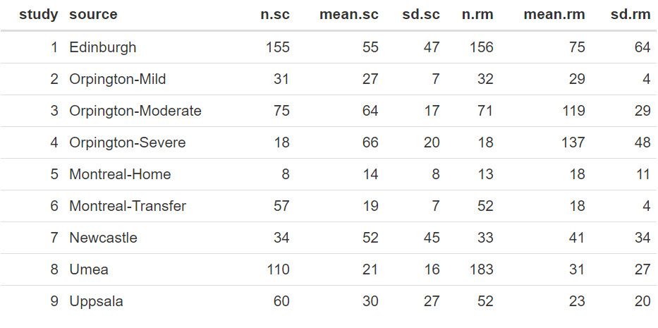
The dataset we will use to illustrate meta-analyses was presented and previously analysed by Normand (1999). The dataset contains infromation from nine independent studies where the length of hospitalisation (measured in days) was recorded for stroke patients under two different treatment regimes. The main objective was to evaluate if specialist inpatient stroke care (sc) resulted in shorter stays when compared to the conventional non-specialist (or routine management) care (rm).

The complete dataset is presented below, and it can also be found in the file STROKE.txt. In this table, the columns present for each study are the sample size (n.sc and n.rm), their estimated mean value (mean.sc and mean.rm) together with their standard deviation (sd.sc and sd.rm) for both the specialist care and routine management care, respectively.

Statistical analyses

We will use the statistical package R to read and manipulate the data, and then the library ASReml-R (Butler et al. 2017) to fit the models. 
First, we read the data in R and make some additional calculations, as shown in the code below:

The new column diff contains the difference between treatment means (as reported from each study). We have estimated the variance of this mean difference, Vdiff, by taking from each treatment its individual MSE (mean square error) and dividing it by the sample size, and then summing the terms of both treatments. This estimate assumes, that for a given study, the samples from both treatments are independent, and for this reason we did not include a covariance. Finally, we have calculated a weight (WT) for each study as the inverse of the variance of the mean difference (i.e., 1/Vdiff).

We can take another look at this data with these extra columns:

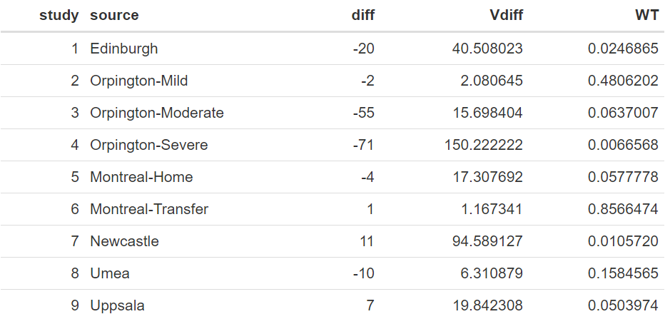
The above table shows a wide range of values between the studies in the mean difference of length of stay between the two treatments, ranging from as low as −71.0 to 11.0, with a raw average of −15.9. Also, the variances of these differences vary considerably, which is also reflected in their weights.

Fitting the model with ASReml-R

The code to fit the fixed-effect linear model using ASReml-R is shown below:

In the above model, our response variable is diff, and the weights are indicated by the variate WT. As the precisions are contained within the weights the command family is required to fix the residual error (MSE) to exactly 1.0, hence, it will not be estimated.

The model generates output that can be used for inference. We will start by exploring our target parameter, i.e. θ, by looking at the estimated fixed effect mean and its standard error. This is done with the code:

Resulting in the output:

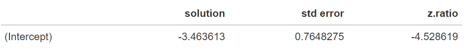
Interpreting results: Fixed-effect model

The estimate of θ is equal to −3.464 days, with a standard error of 0.765. An approximate 95% confidence interval can be obtained by using a z-value of 1.96. The resulting approximate 95% confidence interval [−4.963;−1.965] does not contain zero. The significance of this value can be obtained by looking at the approximated ANOVA table using the command:

Note that this is approximated as, given that weights are considered to be known, the degrees of freedom are assumed to be infinite; hence, this will be a liberal estimate.

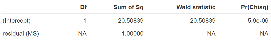
The results from this ANOVA table indicate a high significance of this parameter (θ) with an approximated p-value of < 0.0001. Therefore, in summary, this fixed effect model analysis indicates a strong effect of the specialised care resulting in a reduction of approximately 3.5 days in hospitalisation.

However, as indicated earlier, a random-effects model might seem more reasonable given the inherent differences in the studies under consideration. Here, we extend the model to include the random effect of study. In order to do this, first we need to ensure that this is treated as a factor in the model by running the code:

The LMM to be fitted using ASReml-R is:

Note in this example the only difference from the previous code is the inclusion of the line random=~study. This includes the factor study as a random effect. An important result from running are the variance component estimates. These are obtained with the command:

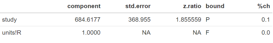
The case for random-effects model

In this example, the variance associated with the differences in the target parameter (θ) between the studies is 684.62. When expressed as a standard deviation, this corresponds to 26.16 days. Note that this variation is large in relation to the scale of the data, reflecting large differences between the random sample of studies considered in the meta-analysis.

We can output the fixed and random effects using the following commands:

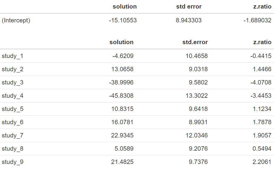
Note that now that our estimated mean difference corresponds to −15.106 days with an standard error of 8.943, and that the approximate 95% confidence interval [−32.634;2.423] now contains zero. An approximated ANOVA based on the following code:

results in the output:

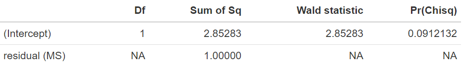
Assessing significance and confidence

We have a p-value of 0.0912, indicating that there is no significant difference in length of stay between the treatments evaluated. Note that the estimates of the random effects of study, also known as BLUPs (best linear unbiased predictions) are large, ranging from −45.8 to 22.9, and widely variable. The lack of significance in the random-effects model, when there is a difference of −15.11 days, is mostly due to the large variability of 684.62 found between the different studies, resulting in a substantial standard error for the estimated mean difference.

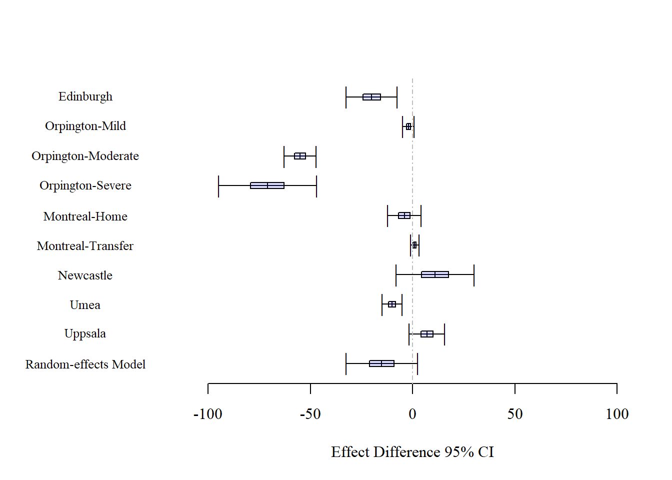
In the following graph we can observe the 95% confidence intervals for each of the nine studies together with the final parameter estimated under the Random-effects Model. Some of these confidence intervals contain the value zero, including the one for the random-effects model. However, it can be observed that the confidence interval from the random-effects model is an adequate summarization of the nine studies, representing a compromising confidence interval.

An important aspect to consider is the difference in results between the fixed-effect and the random-effects model that are associated, as indicated earlier, with different inferential approaches. One way to understand this is by considering what will happen if a new random study is included. Because we have a large variability in the study effects (as denoted by ), we expect this new study to have a difference between treatments that is randomly within this wide range. This, in turn, is expressed by the large standard error of the fixed effect θ, and by its large 95% confidence interval that will ensure that for ‘any’ observation we cover the parameter estimate 95% of the time. Therefore, as shown by the data, it seems more reasonable to consider the random-effects model than the fixed-effect model as it is an inferential approach that deals with several sources of variation.

Making informed decisions in meta-analysis

In summary, we have used the random-effects model to perform meta-analysis on a medical research question of treatment differences by combining nine independent studies. Under this approach we assumed that all studies describe the same effect but we allowed for the model to express different effect sizes through the inclusion of a random effect that will vary from study to study. The main aim of this analysis was not to explain why these differences occur, here, our aim was to incorporate a measure of this uncertainty on the estimation of the final effect of treatment differences.

There are several extensions to meta-analysis with different types of responses and effects. Some of the relevant literature recommended to the interested reader are van Houwelingen et al. (2002) and Vesterinen et al. (2014). Also, a clear presentation with further details of the differences between fixed-effect and random-effects models is presented by Borenstein et al. (2010).

Files to download

Dataset: STROKE.txt
R code: STROKE_METAA.R

References

Borenstein, M; Hedges, LV; Higgins, JPT; Rothstein, HR. 2010. A basic introduction to fixed-effect and random-effects models for meta-analysis. Research Synthesis Methods 1: 97-111.

Butler, DG; Cullis, BR; Gilmour, AR; Gogel, BG; Thompson, R. 2017. ASReml-R Reference Manual Version 4. VSNi International Ltd, Hemel Hempstead, HP2 14TP, UK.

Normand, ST. 1999. Meta-analysis: Formulating, evaluating, combining, and reporting. Statistics in Medicine 18: 321-359.

van Houwelingen, HC; Arends, LR; Stignen, T. 2002. Advanced methods in meta-analysis: multivariate approach and meta-regression. Statistics in Medicine 21: 589-624.

Vesterinen, HM; Sena, ES; Egan, KJ; Hirst, TC; Churolov, L; Currie, GL; Antonic, A; Howells, DW; Macleod, MR. 2014. Meta-analysis of data from animal studies: a practical guide. Journal of Neuroscience Methods 221: 92-102.

About the author

Salvador Gezan is a statistician/quantitative geneticist with more than 20 years’ experience in breeding, statistical analysis and genetic improvement consulting. He currently works as a Statistical Consultant at VSN International, UK. Dr. Gezan started his career at Rothamsted Research as a biometrician, where he worked with Genstat and ASReml statistical software. Over the last 15 years he has taught ASReml workshops for companies and university researchers around the world. 

Dr. Gezan has worked on agronomy, aquaculture, forestry, entomology, medical, biological modelling, and with many commercial breeding programs, applying traditional and molecular statistical tools. His research has led to more than 100 peer reviewed publications, and he is one of the co-authors of the textbook “Statistical Methods in Biology: Design and Analysis of Experiments and Regression”.