Unlocking insights from multi-centre clinical trials: A guide to linear mixed model analysis

The role of multi-centre trials in clinical research

Clinical trials are often conducted across multiple centres, because there are a limited number of suitable experimental subjects in each centre or to include subjects from a wider demographic range (e.g., geographic location, economic group, ethnicity, age, etc.). Subsequent analysis of data from a multi-centre trial must consider the possibility of differences between the individual centres and their effect on treatment. Ignoring centre effects in the analysis makes the implicit (and usually incorrect!) assumption that all centres are identical to one another. In a linear mixed model (LMM) analysis, between-centre differences can be easily accounted for, resulting in more reliable estimates of the treatment effects.

Linear mixed model analysis for multi-centre trials

When LMMs are used to analyse data from a multi-centre trial, assessment of the treatment effects across centres is possible. However, we must decide whether centre and the centre by treatment interaction are fitted as fixed or random terms, since this will affect the interpretation of our results: when fitted as fixed, inference can only be made about the centres observed, but if fitted as random, inference can be applied to the wider population of centres. 

Example: A multi-centre trial of treatments for hypertension

Let’s look at an example: “A multi-centre trial of treatments of hypertension” from the book Applied Mixed Models in Medicine by Brown and Prescott. 

The data is from a study to compare three drug treatments (A, B, and C) for controlling hypertension. Twenty-nine medical centres participated in the trial and the drug treatments were randomly assigned to the patients. Diastolic blood pressure was recorded for each patient pre-treatment (dbp1) and post-treatment (dbp). The main objective of this trial was to assess the effect of the three treatments on diastolic blood pressure. You can download the data here: dbp_finalvisit.txt.

The first few rows of the data are shown below:

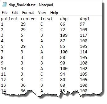
Note: patient, centre, and treat are factors whilst dbp and dbp1 are variates

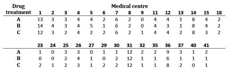
The following table gives the number of patients in drug treatment group A, B or C at each centre in the dataset. Notice that the data are unbalanced, and not all centres had patients on all three drugs.

The full model for analysing this data includes the baseline (i.e., pre-treatment) diastolic blood pressure (dbp1) as a covariate, treatment (treat) as a fixed term, and centre and the centre-by-treatment interaction (centre.treat) as either fixed or random terms:  

where		=	post-treatment diastolic blood pressure for patient k, receiving treatment j at centre i
		=	intercept
		=	baseline covariate effect
		=	baseline diastolic blood pressure for patient ijk
		=	(fixed or random) effect of the ith centre
		=	fixed effect of the jth treatment
		=	(fixed or random) interaction effect between jth treatment at the ith centre
		=	residual error for patient ijk

and the residual error () is assumed to have a Normal distribution with mean zero and variance (i.e., ~ N (0, )). 

Fitting models with fixed terms: Results and interpretations

In the model above, when centre and the centre.treat are as random terms, it is also assumed that the centre and centre.treat effects arise from Normal distributions with mean zero and variances and , respectively. 

Both models are easily fitted in ASReml-R4 and Genstat. In this blog, we’ll use ASReml-R4. However, you can learn how to fit these models in Genstat by watching this short YouTube video: Genstat: Mixed mode for clinical data. 

We’ll begin by fitting the model with both centre and centre.treat as fixed terms: ASReml-R4 code for fitting this model is:

Note, in this model the residual is the only random term. The estimated residual variance ) and its standard error are given below:

The Wald tests for the fixed effects are:

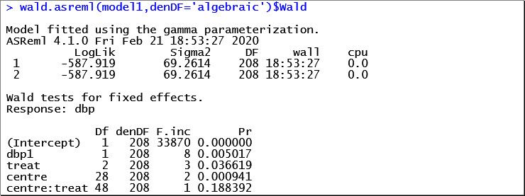
Notice that the centre-by-treatment interaction (denoted by centre:treat) is not statistically significant (p = 0.1884). Therefore, we’ll output just the means and standard errors  for the treatment factor.

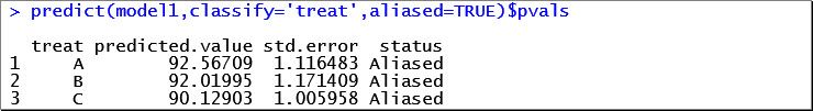
Note: the aliasing has occurred because not all centres had patients on all three drugs. That is, there are missing combinations of centre-by-treatment.

Alternatively, let’s fit centre and the centre-by-treatment interaction as random terms.  The ASReml-R code for this model is:

The estimated variance components and estimated fixed effects are given below:

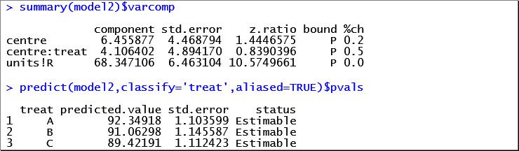
Compared to the first model with fixed effects for centre and centre-by-treatment, we have assumed that differences between treatments vary randomly between the centres. This enables us to draw conclusions about the entire population of centres, rather than just the 29 observed.

ASReml-R4: A powerful tool for linear mixed model analysis

Linear mixed models are fitted using a method known as residual maximum likelihood (REML). The ASReml-R4 package is specially designed for fitting linear mixed models using REML. It is a rich and flexible tool for the analysis of many data sets arising in animal, plant and aqua breeding, agriculture, environmental sciences, and medical sciences.

Genstat: A versatile statistics software package

Genstat is a general statistics software package for education and research. Flexible and easy-to-use Genstat may be applied to any field of research. The user interface contains comprehensive menus to guide non-technical users to use statistics correctly and effectively. It also has a powerful programming language that can be used to develop new techniques and complex experiments. Genstat provides a huge range of statistical procedures, data management, and graphical capabilities. 

Reference

Brown, H. and Prescott, R. (2015). Applied Mixed Models in Medicine. Third Edition. John Wiley & Sons Ltd, England.