Deciding which variables matter: exploring multiple linear regression in Genstat

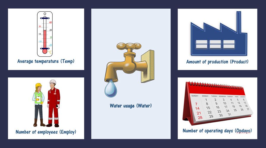
The general aim of regression is to model the relationship between a response variable (y) and one or more explanatory variables (x variables). However, when we have several explanatory variables, this creates an extra challenge: we need to decide which explanatory variables to include in our model.  That is, we need to explore the different possible models by comparing alternative explanatory variables or sets of explanatory variables.  We can do this by:

1. manually fitting a sequence of regression models,
2. performing all subsets regression, or
3. using stepwise regression.

Each of these approaches involves fitting a series of different models, which will then need to be assessed and compared. There are many different statistics to compare models; for example, two of the most used goodness-of-fit (GOF) statistics are the adjusted R-squared (here, we select the model with the largest value) and the mean square error (here, we select the model with the smallest value). We will not go into detail about the different GOF statistics here, but Genstat has several options available.

Let’s see how Genstat can help us select which variables to include in our regression using these different approaches.

Consider the following scenario[i]:

Manually fitting a sequence of regression models

As the name suggests, this approach involves manually adding or dropping explanatory variables. It is a useful approach when we have a good understanding of the process under study and when we are only dealing with a few explanatory variables.

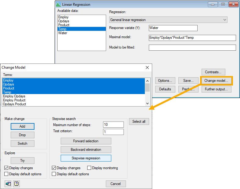
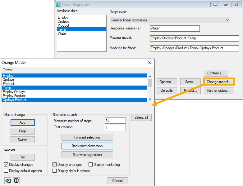
Opened by clicking the Change model button on Genstat’s Linear Regression menu after an initial Run, the Change Model menu allows us to change our current model by adding or removing explanatory variables from it.  The change in mean square error (with accompanying F-test) and the change in percentage variance explained (c.f. adjusted ) can be used to compare our current model with the modified one.   

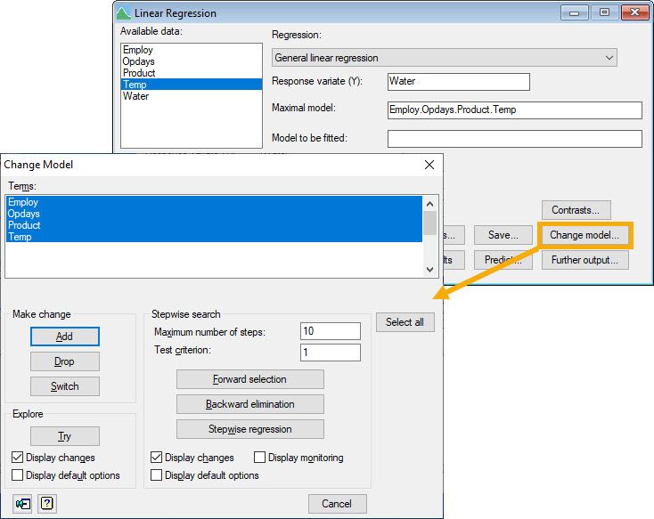Menu: Stats | Regression Analysis | Linear Models… (General linear regression)

• Add adds the selected terms (i.e., explanatory variables) to the model.
• Drop removes the selected terms from the model.
• Switch removes all terms in the current model and adds those that were not included.
• Try allows you to assess the effect of switching (i.e., adding or dropping) each of the terms selected without actually changing your current model.

Exploring all subsets regression: uncovering patterns

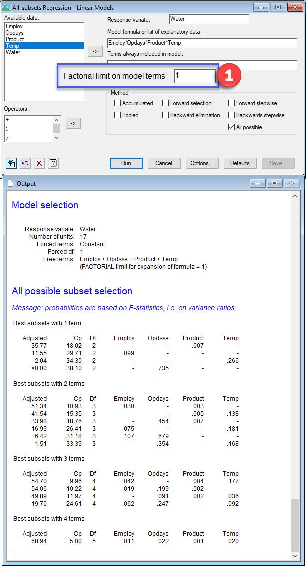
An alternative approach that eliminates some of the subjectivity of the manual option is to consider every combination of explanatory variables. This is known as all subsets regression. Here, we search through all possible linear regression models and compare them using some selection criterion. However, fitting all possible regression models can be very computer intensive! This is especially a concern when you have lots of explanatory variables. Furthermore, it should be used with caution because it allows you to select models that appear to have a lot of explanatory power but contain only noisy variables (a phenomenon known as over-fitting).

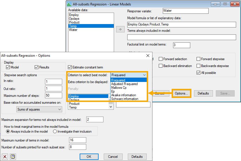Menu: Stats | Regression Analysis | All-subsets Regression | Linear Models…

Stepwise regression: automatic selection

Finally, it is possible to instruct the software to follow an automated stepwise process where only the best (or worst) explanatory variables are added to (or dropped from) the model according to our chosen test criterion. This approach is recommended when you have a large number of explanatory variables to evaluate. The stepwise facilities in the Change Model menu of Genstat are used to build up the regression model automatically.

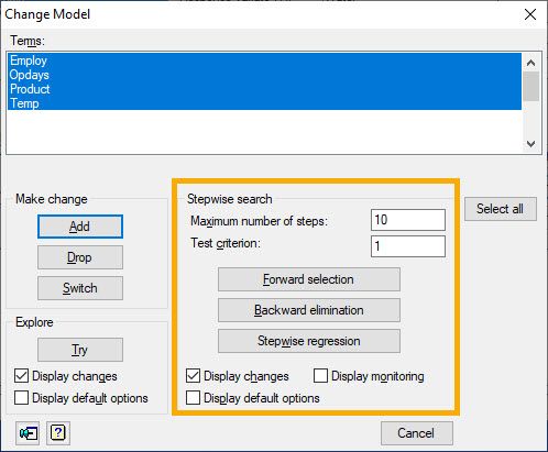
• Forward selection builds a regression model by adding explanatory variables sequentially. In each forward step, the variable that gives the largest improvement to the model is added. (That is, the variable that results in the lowest mean square error provided that its variance ratio exceeds the value specified in the Test criterion box.)
• Backward elimination builds a regression model by removing explanatory variables sequentially. In each elimination step, the variable that results in the smallest decrease in improvement to the model is dropped. (This is the variable with the smallest variance ratio provided it doesn’t exceed the value specified in the Test criterion field.)
• Stepwise regression builds a regression model by sequentially dropping and adding explanatory variables. That is, it switches from forward selection to backward elimination several times before arriving at the final model according to the specifications in the Test criterion field.

Choosing the right model

All of the above approaches are easily implemented in Genstat, and Genstat will provide you with concise output so that you can easily compare models and select a reasonable one. However, you should remember that many models are likely to have a similar GOF statistic, and you must select the one that is most sensible for your study. This involves considering the:

• interpretability of the model (i.e. we should include variables and combination of variables that make sense),
• simplicity of the model (i.e. the principle of parsimony means that we should favour models with fewer variables), and
• the fit of the model (i.e. does the model provide a reasonable fit to the data and do the model assumptions hold?).

Always remember the famous saying: “All models are wrong, but some are useful”!

You might wonder now which one is the “best” model for this water usage study. We chose the model containing all four of the explanatory variables (Employ+Opdays+Product+Temp) plus the interaction Opdays.Product. These are the steps we took to arrive at this model:

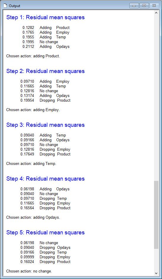
Step 1: We used stepwise regression to explore which explanatory variables to include as additive terms in the model (that is, we didn’t consider interactions between the explanatory variables in this step).

The analysis indicated that we should include the main effects of all four explanatory variables.

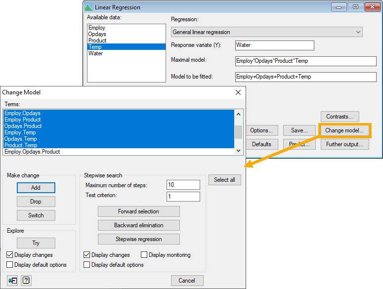
Step 2: We used stepwise regression to explore which 2-way interactions to include in the model already containing the main effects of the four explanatory variables. The analysis indicated that we should include the interaction between the number of operating days (Opdays) and the amount of production (Product).

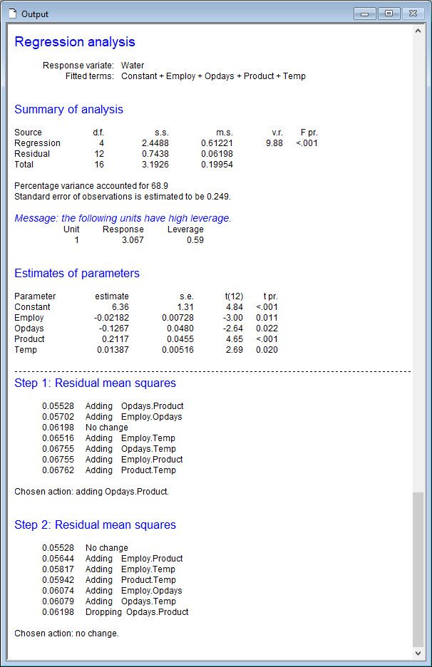
Step 3: We used backwards elimination to assess whether we could simplify the model by dropping either the interaction (Opdays.Product) or the main effects of Employ (number of employees) or Temp (Average temperature) from the model. Note, when an interaction is included in a model, the main effects comprising it should also be included.  Therefore, during this elimination step we did not test the main effects of Opdays or Product).

As the analysis indicated that we should not eliminate any of the current explanatory variables from our model, we stopped here and selected the model with the explanatory terms: Employ + Opdays + Product + Temp + Opdays.Product.

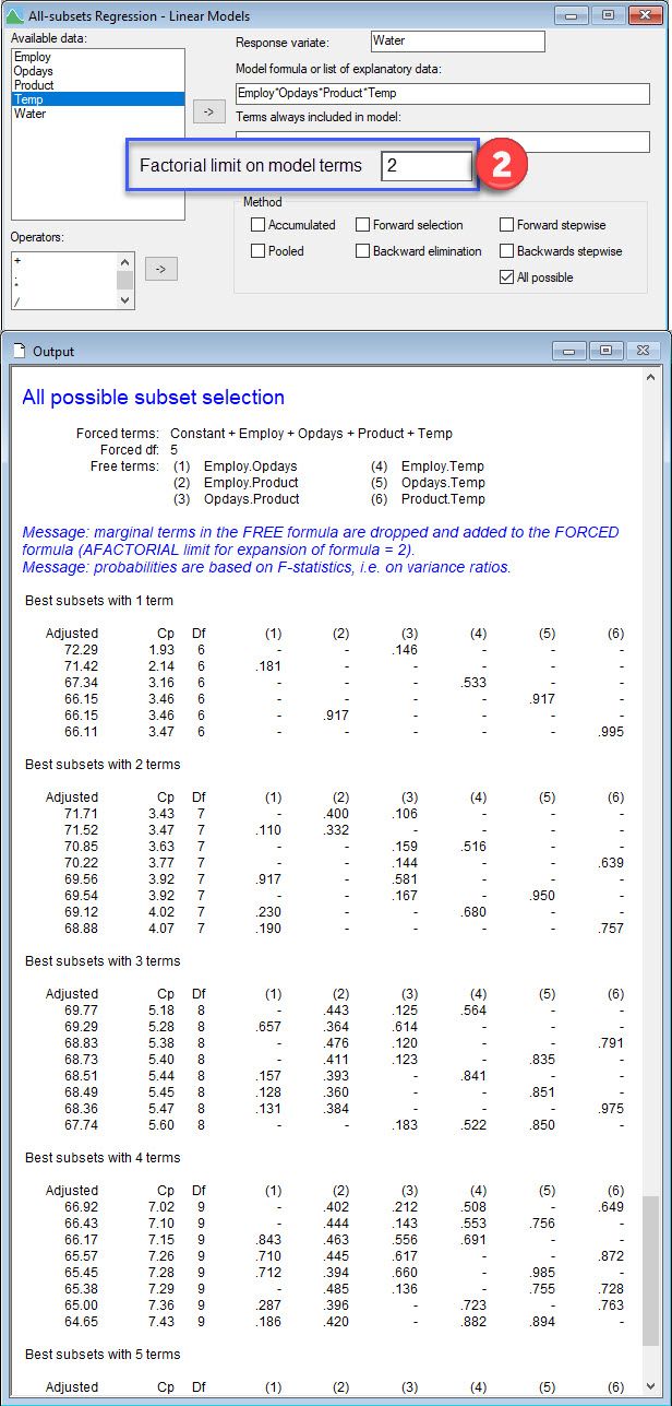
Note, all subsets regression, where adjusted is used to compare models, leads to the same model selected.  Comparing all the additive models shows that the one containing all four explanatory variables has the highest adjusted , 68.94%.  Then, comparing the set of models with 2-way interactions in addition to the four main effects, we learn that the model now with the highest adjusted (72.29%) also contains the Opdays by Product interaction.

Comparing additive models

Adding 2-way interactions

You can learn more about multiple linear regression in the Genstat Regression Guide (Help | Genstat Guides | Regression → Multiple linear regression, p.17-29).

[i] This example originated from Draper and Smith (1998, Applied Regression Analysis, p. 355), and the data can be accessed in Genstat by selecting File | Open Example Data Sets | Water.gsh.