' fill='none' stroke='%23304560' stroke-miterlimit='10' stroke-width='2'/%3e%3c/svg%3e)

Paired data: What is it and how is it analysed?
The VSNi Team
26 January 2022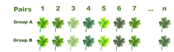
With paired data, every observation in one group has a matching observation in the other group. These could be different observations on the same subject, as in a “before and after” scenario, or they could be observations on different subjects where the subjects have been paired based on some important underlying characteristic (e.g., age, genetic relatedness, health status, geographic location, etc.). Paired data is a special case of a randomized complete block design (RCBD) in which there are only two treatment conditions and subjects can be grouped into homogenous pairs prior to treatment.
Let’s look at an example of paired data.
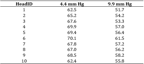
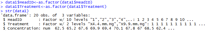
The data set below is from an experiment on red clover to investigate the effect of vapour pressure on the sugar concentrations of the nectar. Ten flowering red clover heads (HeadID) were divided in half; one half was randomly subjected to a vapour pressure of 4.4 mm Hg, the other to a vapour pressure of 9.9 mm Hg. Sugar concentrations of nectar in half heads of the red clover were kept at different vapour pressures for eight hours (Steel and Torrie, page 103). The data set, therefore, contains 10 pairs of observations: the 2 sugar concentration measurements (one at each level of the pressure treatment) on the same red clover head. This data is shown in the table below.
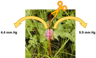
Importantly, the two halves of the clover head are related; we would expect them to respond to the same treatment in the same way. In addition, we would expect them to have very similar nectar sugar concentrations pre-treatment. That is, the pairs of observations are not independent, and this must be taken into account in the analysis. If analysed correctly, this pairing eliminates inherent differences between the experimental units (i.e., head halves), giving us more power to detect real treatment differences.
In this blog, we’ll demonstrate how the dependence between pairs of observations is taken into account in a linear mixed model (LMM). However, paired data like this can also be analysed using a paired t-test. To find out more, refer to the Note on t-tests at the end of this blog, or watch the Genstat YouTube video Paired t-test and Wilcoxon matched-pairs test.
Transforming the data into long format
First, let’s reshape the data into long-format by stacking the data and creating a factor for the pressure treatment. You can do this in R using the following code.
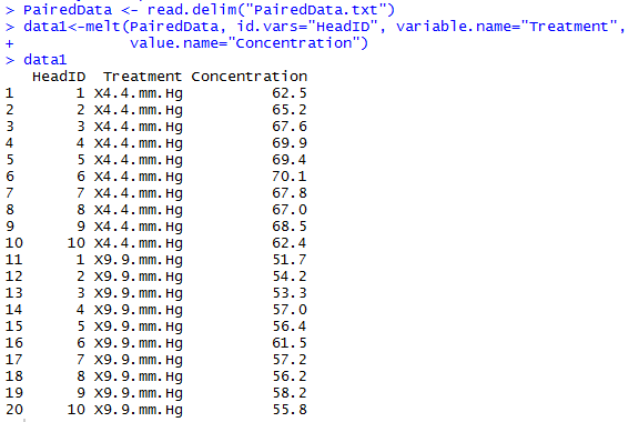
Both HeadID and Treatment should be factors, whilst Concentration is our response variate. This is defined in the first two lines of the following:
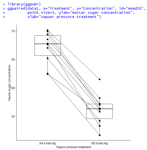
In the following plot, the nectar sugar concentrations are plotted for the two vapour pressure treatments. Lines connect the two observations from the same red clover head. Of interest is whether the mean nectar sugar concentration differs between the two treatments. We’ll examine this by fitting a LMM.
The LMM for the analysis of our paired data includes Treatment as a fixed term and HeadID as a random term. Importantly, the dependence (i.e., correlation) between the pair of observations originating from the same red clover head is accounted for by the HeadID random term.
The ASReml-R 4 and nlme codes for fitting this model are shown below, followed by their results:
ASReml-R 4
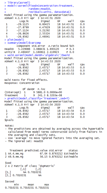
library(asreml)
m_asreml <- asreml(fixed=Concentration~Treatment,
random=~HeadID,
data=data1)
Nlme
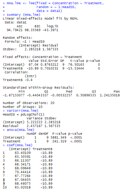
library(nlme)
m_nlme <- lme(fixed=Concentration~Treatment,
random=~1|HeadID,
data=data1)
Let’s examine the ASReml-R 4 output in more detail.
Evaluating residuals for assumptions
ASReml-R 4 provides four different residual diagnostic plots. These are useful for checking the residual assumptions of normality and constant variance.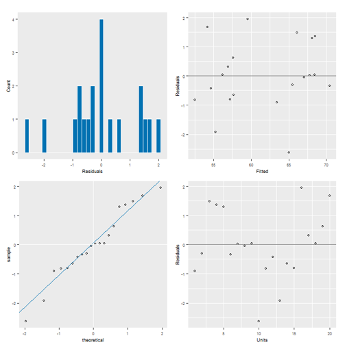
For normality:
- The histogram (top left) should have a reasonably symmetric bell-shape.
- The normal plot (bottom left) should form approximately a straight line.
For constant variance:
- The spread of the residuals in the scatterplots against: i) fitted values (top right) and ii) units (bottom right) should be roughly equal over the range of the data.
The residuals from our model appear to be acceptable.
Estimating random variance components
The estimated variance component for HeadID is 5.23, with a standard error of 3.09. For the residual error (units!R) the estimated variance component is 2.46, with a standard error of 1.16.
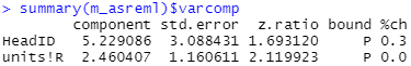
Conducting Wald tests for fixed effects
The Wald test (which is equivalent to an ANOVA, but in the context of LMM) provides strong statistical evidence of a Treatment effect (P < 0.001). That is, we have evidence that the mean nectar sugar concentrations differ between the two vapour pressure treatments.
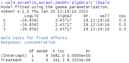
Determining treatment means and standard errors
It is also possible to obtain with ASReml-R 4 treatment means and their standard errors. The mean nectar sugar concentration for red clover heads subjected to a vapour pressure of 4.4 mm Hg is 67.04, whereas at 9.9 mm Hg it is 56.15. The standard error of these means is 0.88, and the standard error of the difference between these means is 0.70.
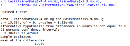
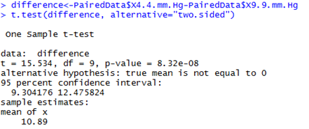
Alternative approaches: T-tests and their limitationsThe vapour pressure treatment means may also be compared using a two-sided paired t-test with a pooled variance as shown below. It may also be compared using a two-sided one-sample t-test on the difference between the paired observations.
Note: By calculating the difference we are effectively eliminating the dependency that existed between the pairs of observations. It is important to note that for all three tests we have 9 degrees of freedom and not 18! This is because we really only have 10 independent pairs of information (i.e., the 10 clover heads) and not 20 pieces of information. This is a critical aspect to consider whenever you have paired or correlated data. The results of the t-tests are equivalent, and in this case identical, to those of LMM above. This is because the data is fully balanced (every clover head has exactly two observations) and there are no other factors or covariates of interest. In more complicated situations however, the simple t-test won’t be appropriate, and you’ll need to take an LMM approach. |
Popular


Related Reads