Exploring spatial modelling: Enhancing statistical analysis for scientists and statisticians

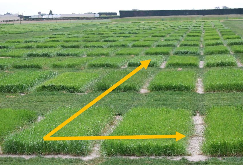
The need to model spatial correlations between observations in two-dimensions occurs when the experimental units are laid out in a grid, for example in a field trial or greenhouse, and experimental units that are closer together experience more similar environmental conditions than those which are further apart. The goal of spatial modelling is to describe how the lack of independence between measurements changes as their separation in space increases or decreases. Importantly, fitting an appropriate spatial model typically improves the estimation of the fixed (or random) treatment effects by modelling more accurately the spatial distribution of the residual effects.

Let’s look at an example.

Constructing an appropriate linear mixed model

The example we’re going to consider is from a field trial to compare the yield of 25 varieties of barley (Gilmour, Thompson and Cullis, 1995). The aim of the trial was to compare the mean yields of the 25 barley varieties. The trial design is a balanced lattice square with 6 replicates, arranged in a 15 column by 10 row grid of plots.

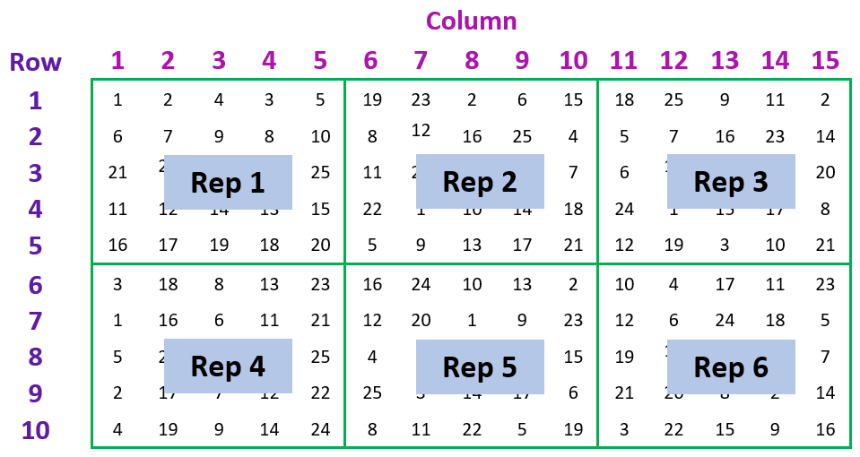
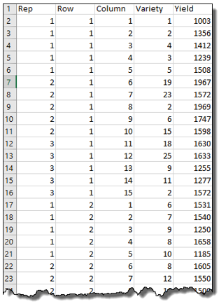
The data contains three factors related to the experimental design: Rep, Row and Column; one factor representing the treatment: Variety; and the response variate: Yield.

Our goal is to estimate and compare the mean Yield of the 25 wheat varieties. However, as this is spatial data, we need to consider potential spatial correlation between observations. That is, the lack of independence between experimental units due to spatial proximity. Linear mixed models provide a powerful framework for analysing spatial data like this. Let’s formulate an appropriate linear mixed model for this spatial data set.

Our Response variate is, of course, Yield, and the fixed model comprises a term for Variety. Now, the random model should include the terms involved in the allocation and randomization of the varieties. For this trial, the allocation of the varieties to positions in the field depended on the blocking structure of the balanced lattice design. As each replicate has a block structure of rows crossed with columns our random model must contain Rep plus Row within Rep (i.e., Rep.Row) plus Column within Rep (i.e., Rep.Column).

Unveiling the intricacies of spatial correlation

Now let’s model the spatial correlation; that is, the lack of independence between experimental units due to spatial proximity.

Spatial correlation is imposed by specifying the appropriate correlation structures on the residual Row by Column term. (Note that each combination of the Row and Column factors represent a unique position in the spatial grid.)  We have many choices of correlation structure, but commonly used ones are:

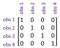
• The identity correlation structure. This assumes that the observations are uncorrelated, or independent of one another, no matter how close they are in space.

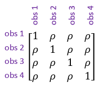
• Simple correlation structure, also known as uniform correlation. This model assumes the correlation (ρ) between measurements is constant regardless of how far apart in space they are.

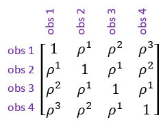
• Autoregressive model of order 1. This model allows the correlations between measurements to decrease as the distance between them increases.

Note: The general correlation structure can be used for both equally and irregularly spaced measurements, whereas the autoregressive correlation structure should only be fitted to equally spaced measurements.

Popular correlation structures: insights and options

In most cases, it is reasonable to expect that the correlation between pairs of experimental units in the spatial grid will decrease the further apart they are. Such a correlation pattern can be modelled by fitting an autoregressive model of order 1 in the row and column directions. This corresponds to an AR1 ⊗ AR1 separable correlation model.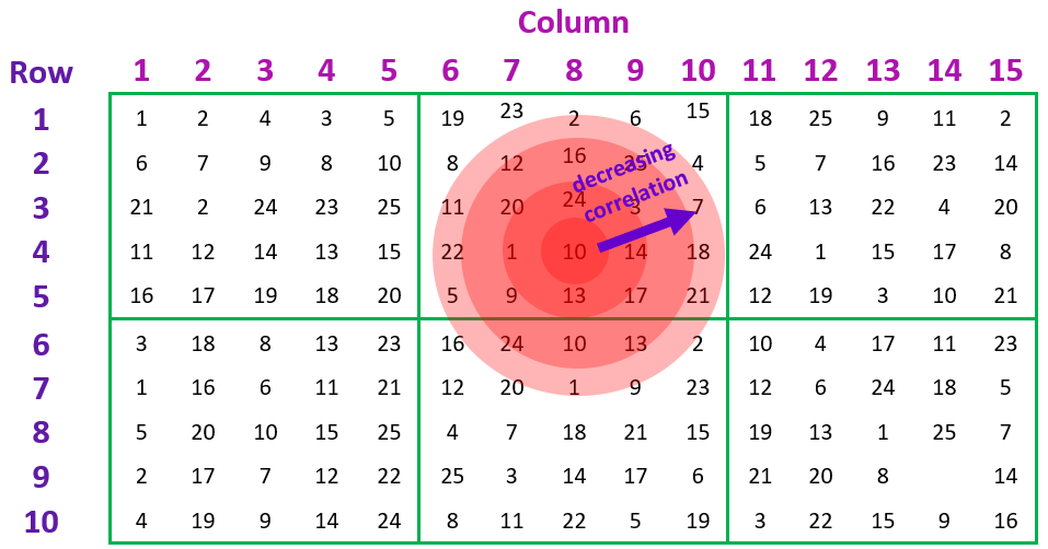

Beyond convention: alternative spatial models explored

However, this is by no means the only spatial model possible. For example, we may discover that the correlation between pairs of experimental units decreases along the columns the further apart they are, but measurements down the rows are uncorrelated. Such a scenario could be modelled by fitting the identity model in row direction and an autoregressive model of order 1 in the column direction. That is, an I ⊗ AR1 separable correlation model.

Factoring in measurement error: capturing grid variability

Measurement error (also known as a nugget effect) is also often needed to represent the variability over the spatial grid correctly. That is, the data may be more variable than what can be accounted for by the spatial model alone. Measurement error is allowed for in a linear mixed model by including an additional random term that indexes the observational units.