' fill='none' stroke='%23304560' stroke-miterlimit='10' stroke-width='2'/%3e%3c/svg%3e)

Which-won-where? GGE biplots in Genstat
The VSNi Team
03 August 2021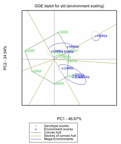
As soon as we get plant breeding data from a multi-environment trial (MET), we start asking the question, “which genotypes perform best in which environments?” - Which-won-where? As it is virtually impossible to make sense of hundreds of numbers in a spreadsheet, we need statistical tools to summarize our MET data and gain better insights. Also, we will probably want to understand the nature of genotype-by-environment (G×E) interaction so we can respond to it or even take advantage of it. GGE biplots are a very powerful and popular visualisation tool for exploring the G×E interaction and for investigating the phenotypic performance of genotypes in different environments.
Multi-environment trials and Gx£A multi-environment trial (MET) comprises a series of experiments conducted over a range of environmental conditions (usually a combination of seasons and geographic conditions) where each genotype of interest is evaluated in all (or almost all) of these environments. Plant breeders use MET data to evaluate the phenotypic performance of genotypes (i.e., cultivars or varieties) across a range of environments. However, the relative performance of a given genotype often varies between environments, a phenomenon known as the genotype-by-environment (G×E) interaction. Plant breeders investigate the G×E interaction to identify genotypes that perform well in all environments (i.e., are suitable for broad use) and those with exceptional performance in specific environments (i.e., are well suited for use in certain growing conditions). |
GGE biplotsGenotypic main effect plus Genotype-by-Environment interaction (GGE) biplots are a very useful visualisation tool for investigating the inter-relationship among genotypes, the inter-relationship among environments, and the interaction between genotypes and environments. In brief, the GGE biplot is based on a standard principal components analysis (PCA) of the environment-centred trait means. It provides information on the total genetic variation by approximating the joint effect of the genotype main effect (G) and the genotype by environment (G×E) interaction using scores from the PCA. |
Exploring GGE biplots for genotype and environment relationships
GGE biplots are based on principal components analysis (PCA) of environment-centred trait means, and a standard GGE biplot is generated by plotting the second principal component scores of the genotypes and the environments against their respective scores for the first principal component. However, additional information can be added, and different views can be created, that help to elucidate the genotype and environment relationships.
The Which-Won-Where view
One popular view is which-won-where as it is an effective display for identifying the best performing genotypes in each environment or group of environments (i.e., mega environments). Genstat’s powerful and user-friendly menus make creating GGE biplots, including the which-won-where view, easy. This process is shown below in some screenshots.
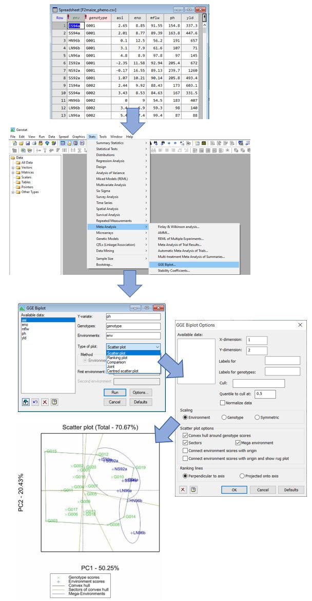
As mentioned above, GGE biplots are created using the trait means (i.e., predictions) for each genotype in each environment. These typically come from a preliminary MET analysis using linear mixed model methodology. Genstat has comprehensive linear mixed model facilities (REML) that provide you with all the statistical tools you need to analyse your MET data and to estimate the trait means needed for your GGE biplot analysis. (For more information see Chapter 4 of the Genstat QTL manual, which is available directly within the Help menu.)
To find out more about creating GGE biplots in Genstat, and also how to interpret them, watch our video.
Popular


Related Reads