' fill='none' stroke='%23304560' stroke-miterlimit='10' stroke-width='2'/%3e%3c/svg%3e)
Calculating Accuracy and Reliability of Random Effect Estimates with ASReml-R

Calculating Accuracy and Reliability of Random Effect Estimates with ASReml-R
An important aim when fitting linear mixed models (LMM) is the use of random effect estimates. In some analyses, such as genetic evaluations, the main objective of the analysis is to obtain these estimates. Random effects, also known as BLUPs (best linear unbiased estimations), are obtained after fitting a LMM, where their variance components are estimated by residual maximum likelihood (REML) and these values are used to calculate BLUPs.
Consider the following LMM for a genetic experiment, where we have a randomized complete block design with blocks and a total of genotypes evaluated:
where is the phenotypic observation of the ith genotype on the jth block; is the overall mean; is the fixed effect of the ith block; is the random effect of the ith genotype, with that is associated with some information about pedigree, from which we can obtain a pedigree-based or genomic-based relationship matrix ; and is the random residual with .
In the above model, also known as Animal Model, the random effects correspond to the breeding value (BV) from which selections of future progenitors or individuals will be done. As these effects are based on estimated variance components, then they are often known as EBVs (estimated breeding values). Statistically, the matrix is critical as it is the place were we specify the correlations or dependencies that exist between random effects.
As many breeding and commercial decisions depend on the EBVs it is important to have an assessment of our confidence in these values, and this is done by calculating a statistical measure of precision. Probably the most common statistic used to assess these effects is the calculation of the correlation between true and predicted random effects, , also known as accuracy. This can be calculated using the following expression for a given genotype as:
This formula requires the PEV (predictor error variance) of , which corresponds to the square of the standard error (SE) of the random effect estimate, i.e. . Most statistical software will report these SE values, including SAS and ASReml. In addition, we have , which is the population estimate of the variance associated with the EBVs, and this is our genetic additive variance, which is used to calculate narrow-sense heritability ().
According to statistical theory, the values of PEV will range from zero to the . In cases where we have full information about a given genotype, then the PEV will be close to zero as we have little uncertainty in the true additive value of a genotype, hence, . However, when there is very little information, then the PEV will approximate to . Note that these extreme values of PEV translate in values of 1.0 and 0.0, respectively. Therefore, values closer to 1.0 are an indication of very good quality of a given additive effect estimate.
Sometimes, you will see reliability instead of accuracy reported, where the former is the square of the later. Both statistics are commonly used when reporting the quality of a random effect estimate in genetic studies.
To illustrate the above calculations, we used genetic data originating from a trial on a population of cultivated two-row spring barley. The original trial measured height (cm) of plants grown in pots during 2011 for a total of 856 lines; however, the available data for this analysis consists of the adjusted mean values of only 478 lines, together with their molecular information. Further details can be found in Oakley et al. (2016).
In our example, we obtained the realized relationship matrix from the single nucleotide polymorphism (SNP) marker information available for these 478 lines, and an Animal Model was fitted considering this genomic matrix. This was done in the package R using the library ASReml-R, and the code used to fit this model was:
modelGBLUP <- asreml(fixed=Hadj11~1,
                     random=~vm(lines, ainv),
                     na.action=na.method(y='include'),
                     data=datagFULL)
Here, the response variable was and our single random effect is the factor that represents our additive effects, and this is associated with the inverse of the relationship matrix . In addition, in the above code it was requested that observations with missing data (i.e., ) in their response variable will be included in the analyses. This allowed us to obtain EBVs for all individuals, even those that were not phenotyped but that were included in the relationship matrix.
The above analysis, using the following code
vc <- summary(modelGBLUP)$varcompwill output the following estimation of variance components.
| component | std.error | z.ratio | bound | %ch | |
|---|---|---|---|---|---|
| vm(lines, ainv) | 34.94159 | 7.880138 | 4.434134 | P | 0.4 |
| units!R | 43.10000 | 7.949305 | 5.421857 | P | 0.0 |
These values correspond to a narrow-sense heritability of for the adjusted mean of height. Hence, the trait has a strong genetic control. Now, we can proceed to request the BLUP (or EBV) values together with their standard errors, this is done using the code:
BLUP <- summary(modelGBLUP, coef=TRUE)$coef.randomBelow we can see a subset of this list with the top 10 and bottom 10 genotypes sorted by their SE values.
| solution | std.error | z.ratio | PEV | accuracy | reliability | |
|---|---|---|---|---|---|---|
| vm(lines, ainv)_LENTA | 5.8347 | 3.9482 | 1.4778 | 15.5885 | 0.7442 | 0.5539 |
| vm(lines, ainv)_PALLAS | 5.1138 | 3.9807 | 1.2846 | 15.8462 | 0.7393 | 0.5465 |
| vm(lines, ainv)_CHARIOT | 1.1494 | 3.9859 | 0.2884 | 15.8871 | 0.7385 | 0.5453 |
| vm(lines, ainv)_CLASS | -7.6429 | 3.9874 | -1.9168 | 15.8990 | 0.7382 | 0.5450 |
| vm(lines, ainv)_BONUS | 7.9205 | 3.9897 | 1.9853 | 15.9176 | 0.7379 | 0.5445 |
| vm(lines, ainv)_TOKEN | -7.8575 | 3.9930 | -1.9678 | 15.9440 | 0.7374 | 0.5437 |
| vm(lines, ainv)_MAJA | 9.9281 | 4.0022 | 2.4806 | 16.0178 | 0.7359 | 0.5416 |
| vm(lines, ainv)_PRESTIGE | -8.4205 | 4.0184 | -2.0955 | 16.1477 | 0.7334 | 0.5379 |
| vm(lines, ainv)_ASPEN | -4.1411 | 4.0456 | -1.0236 | 16.3670 | 0.7291 | 0.5316 |
| vm(lines, ainv)_CORNICHE | -1.6122 | 4.0546 | -0.3976 | 16.4394 | 0.7277 | 0.5295 |
| solution | std.error | z.ratio | PEV | accuracy | reliability | |
|---|---|---|---|---|---|---|
| vm(lines, ainv)_FREJA | 28.0177 | 4.8260 | 5.8056 | 23.2902 | 0.5775 | 0.3335 |
| vm(lines, ainv)_DASIO | -8.5969 | 4.8376 | -1.7771 | 23.4028 | 0.5747 | 0.3302 |
| vm(lines, ainv)_KESTREL | -0.4303 | 4.8644 | -0.0885 | 23.6623 | 0.5682 | 0.3228 |
| vm(lines, ainv)_GAIRDNER | 5.3170 | 4.9188 | 1.0810 | 24.1944 | 0.5546 | 0.3076 |
| vm(lines, ainv)_STELLA | 15.1422 | 4.9273 | 3.0731 | 24.2781 | 0.5524 | 0.3052 |
| vm(lines, ainv)_LOGAN | 5.7601 | 4.9716 | 1.1586 | 24.7170 | 0.5409 | 0.2926 |
| vm(lines, ainv)_CLARA | 9.4874 | 5.3870 | 1.7612 | 29.0197 | 0.4117 | 0.1695 |
| vm(lines, ainv)_MARESI | 1.5449 | 5.7448 | 0.2689 | 33.0032 | 0.2355 | 0.0555 |
| vm(lines, ainv)_FLICK SEJET | -8.5443 | 5.8523 | -1.4600 | 34.2490 | 0.1408 | 0.0198 |
| vm(lines, ainv)_BEKA | 16.5908 | 6.0992 | 2.7202 | 37.2001 | NaN | -0.0646 |
The EBV estimates for this data are positive and negative, as they represent deviations from the overall height mean. For example, the genotype FREJA has an EBV of indicating that, if this parent is crossed with a parent of equal genetic worth, its progeny will have an expected deviation from the mean of cm. The full range of EBVs is between − cm to cm, a wide interval considering that the mean of the population is cm, and this is a result of the relatively large heritability value found for this trait.
Also, there is an interesting range in SE values from to . The width of this range is related to the level of genetic relationships between individuals, that is specified through the matrix . Genotypes with many relatives will share or collect information from many phenotypic responses, and therefore they will have lower SE values; in contrast, individuals with few, or no relatives, will tend to have much higher SE values. However, it is also possible that individuals with no phenotypic data will have large SE values, unless they have many relatives to help with the estimation of their EBVs.
Now, we can proceed to calculate the accuracy and reliability using the expressions shown before, with the code
Va <- vc[1,1]
BLUP$PEV <- BLUP$std.error^2
BLUP$accuracy <- sqrt(1 - BLUP$PEV/Va)
BLUP$reliability <- 1 - BLUP$PEV/Va
And now we can observe these calculated values for a subset of the top 10 and bottom 10 individuals.
| PEV | accuracy | reliability | |
|---|---|---|---|
| vm(lines, ainv)_LENTA | 15.5885 | 0.7442 | 0.5539 |
| vm(lines, ainv)_PALLAS | 15.8462 | 0.7393 | 0.5465 |
| vm(lines, ainv)_CHARIOT | 15.8871 | 0.7385 | 0.5453 |
| vm(lines, ainv)_CLASS | 15.8990 | 0.7382 | 0.5450 |
| vm(lines, ainv)_BONUS | 15.9176 | 0.7379 | 0.5445 |
| vm(lines, ainv)_TOKEN | 15.9440 | 0.7374 | 0.5437 |
| vm(lines, ainv)_MAJA | 16.0178 | 0.7359 | 0.5416 |
| vm(lines, ainv)_PRESTIGE | 16.1477 | 0.7334 | 0.5379 |
| vm(lines, ainv)_ASPEN | 16.3670 | 0.7291 | 0.5316 |
| vm(lines, ainv)_CORNICHE | 16.4394 | 0.7277 | 0.5295 |
| PEV | accuracy | reliability | |
|---|---|---|---|
| vm(lines, ainv)_FREJA | 23.2902 | 0.5775 | 0.3335 |
| vm(lines, ainv)_DASIO | 23.4028 | 0.5747 | 0.3302 |
| vm(lines, ainv)_KESTREL | 23.6623 | 0.5682 | 0.3228 |
| vm(lines, ainv)_GAIRDNER | 24.1944 | 0.5546 | 0.3076 |
| vm(lines, ainv)_STELLA | 24.2781 | 0.5524 | 0.3052 |
| vm(lines, ainv)_LOGAN | 24.7170 | 0.5409 | 0.2926 |
| vm(lines, ainv)_CLARA | 29.0197 | 0.4117 | 0.1695 |
| vm(lines, ainv)_MARESI | 33.0032 | 0.2355 | 0.0555 |
| vm(lines, ainv)_FLICK SEJET | 34.2490 | 0.1408 | 0.0198 |
| vm(lines, ainv)_BEKA | 37.2001 | NaN | -0.0646 |
For this trait, the range of correlation between true and predicted breeding values, , is from to , and the lowest accuracy and reliability values correspond to individuals with the largest SE values. Note that the genotype has a for accuracy, which originates from a negative square root, as this BLUP has an SE that is larger than .
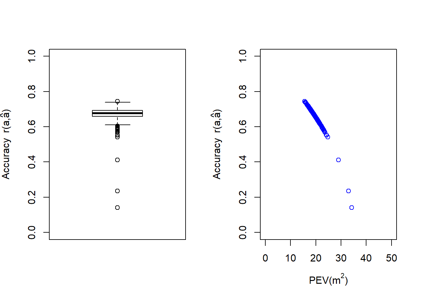
In the above figure we present a boxplot of the accuracy values (left plot) and a scatterplot of the PEV against accuracy (right plot). It is clear from these plots that there is a group of three observations with very poor accuracy that have values lower than . However, the majority of the observations are found with accuracy values of or higher, where some of them reach values as high as .
It is interesting to speculate what the reasons could be for these three lower observations (genotypes , and ) together with the observation (genotype ), to be so different from the rest of the population. The unusual behavior of these four observations is likely to reflect errors in their information, including phenotypic response (maybe a potential outlier), or incorrect genetic relationships (due to pedigree or genotyping errors).
In summary, we have calculated values of accuracy and reliability for the estimation of random effects from an Animal Model. For the data analyzed, these represented a wide range of values, reflecting different levels of precision. For example, a large value of accuracy , such as , will indicate that there is little expected change on the estimation of the EBV if additional information is collected from a given genotype or from its relatives (e.g., its offspring). Therefore, values provide us with a good measure of our confidence in the genetic evaluation performed.
In our analysis, and in many other genetic analyses, it is critical to consider the incorporation of the matrix of genetic relationships, as it will allow us to improve the estimation of the random effects because we have changed our assumption from independent random effects to a model that considers correlations or dependencies between these random effects.
A routine check of the accuracy and reliability (and indirectly of PEV values), can help to make future improvements on the quality of the information obtained from statistical analyses. For example, we can assess the consequences of incorporating additional relatives or replicates in future evaluations. Alternatively, these checks can also help to assess the benefits of using more complex linear models, such as those that combine multiple traits, measurements or sites.
Finally, the above calculations can be extended to any other random effect on all linear mixed models fitted, and their use is recommended to assess the quality of the estimates beyond what a simple standard error will indicate.
Author
Salvador A. Gezan
Reference
Oakey, H; Cullis, B; Thompson, R; Comadran, J; Halpin, C; Waugh, R. 2016. Genomic selection in multi-environment crop trials. Genes | Genomes | Genetics 6:1313-1326
Notes: SAG Jan-2020