' fill='none' stroke='%23304560' stroke-miterlimit='10' stroke-width='2'/%3e%3c/svg%3e)
Likelihood-based Statistical Inference for Variance Components in Linear Mixed Models

Likelihood-based Statistical Inference for Variance Components in Linear Mixed Models
Statistical inference is the process of drawing some conclusions about a population based on the sample data at hand. This is what we do when we fit a linear mixed model to our data, where some population parameters (e.g., treatment means) are estimated and used to draw conclusions about our study. Under statistical inference we want to expand our findings to the complete population from where our data originated.
The three most common types of statistical inference are: 1) point estimation, 2) interval estimation, and 3) hypothesis testing. Point estimation is where we estimate an unknown parameter that is presented as a single numeric value. In contrast, under interval estimation, we represent the estimated unknown parameter using a range of numeric values that is highly likely to contain the true population value. This range is known as the confidence interval. Finally, under hypothesis testing, we assess the evidence provided by the sample data in favor, or against, a given claim about the population. This is usually done using a statistical test.
All of the above types of statistical inference are commonly used for linear mixed models (LMM), and these can be implemented on fixed or random effects, functions of these effects (e.g., predicted means), and variance components or their functions (e.g., heritability).
In this tutorial we will present an example where statistical inference is done for a variance component. In this example, the aim of our LMM is to estimate a correlation variance component (), and we are interested in: 1) knowing what is the value of this correlation (point estimate), 2) reporting a 95% confidence interval (interval estimation), and 3) evaluating if this parameter is significantly different from zero (hypothesis testing).
The dataset used originates from a study that evaluated IQ scores for twins (McClave and Sincich, 2009). In this research, IQ scores of 32 pairs of identical twins were measured, where one of the twins () was reared by their natural parent, and the other () was reared by a relative or another person. Studies with twins are ideal because they share identical genetics, and therefore, their differences will be due exclusively to non-genetic factors, like in this case the type of rearing. For this study, the main objective is to evaluate if there are statistically significant differences between the average IQ scores between these two rearing levels.
The dataset for this example can be found at the end of this document in the file . The first few lines are:
| PairID | TwinR | IQ |
|---|---|---|
| 112 | A | 113 |
| 112 | B | 109 |
| 114 | A | 94 |
| 114 | B | 100 |
| 126 | A | 99 |
| 126 | B | 86 |
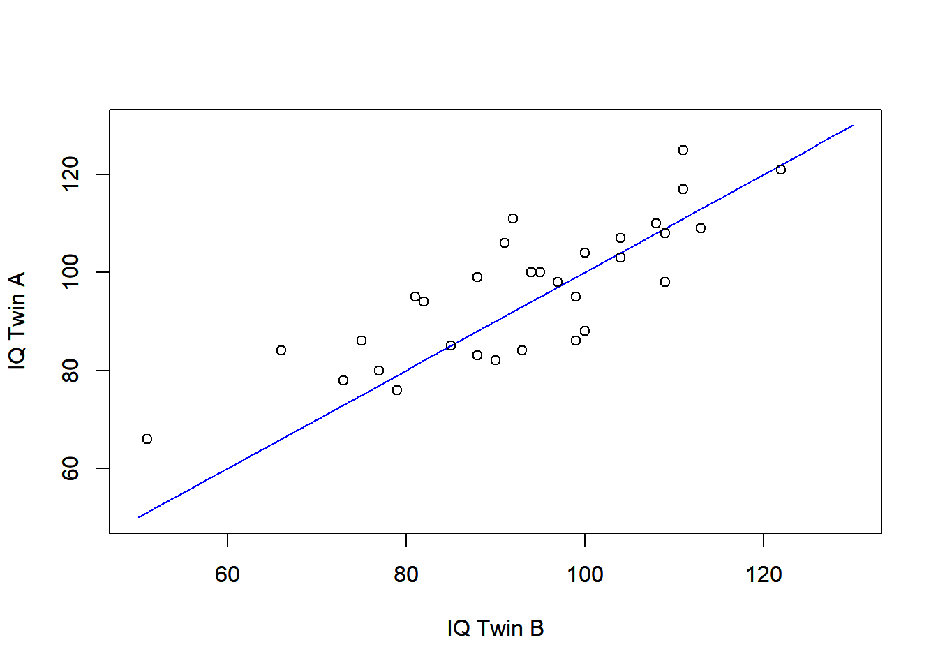
Here, we have a factor that identifies the pair of twins , and another that specifies the rearing type ( = reared by neutral person, = reared by relative or other person). The raw means (and standard deviations) for groups and are 93.22 (15.17) and 96.13 (13.66), respectively. These values indicate small differences in IQ between these groups. In addition, we can also plot the IQ scores for each pair of twins, as shown in the below. We note a reasonable relationship between the IQ scores from the same twin pair, with a Pearson’s correlation of 0.816.
Now, let’s fit our LMM. First, we will define our model in a generic way:
where is the IQ measurement for the ijth twin; is the fixed effect of rearing type ( or ), and is the residual error, with .
For analysis, the above model needs to indicate that the errors, , are not independent from each other. In this case we need to specify that observations belonging to the same twin pair are correlated. This will be done in ASReml-R by a using the variance component structure . For a single twin pair this structure has the following form:
This variance structure is described by 2 variance components, one associated with the error variance, , and the other, , representing the correlation between residual errors of the same twin pair. It is important to note that these parameters have natural constraints: can only be positive, and has to be between -1 and +1.
In ASReml-R we can fit this model and produce basic output using the following code:
modT<-asreml(fixed=IQ~TwinR,
             residual=~id(PairID):corv(TwinR),
             data=TWINS)
predict(modT,classify='TwinR')$pvals
wald.asreml(modT,denDF='numeric')$Wald
summary(modT)$varcomp
The above model has the fixed effect of , but under we have defined a matrix of variance-covariance between all residuals. Here, we have an identity matrix of dimension 32 × 32 () multiplied (using the Kronoecker product, ) by a 2 × 2 matrix () defined as above. Therefore, this forms a matrix of dimension 64 × 64 corresponding to the number of observations in the dataset, as shown below.
After fitting this model, we obtain a log-likelihood value of -183.650, and the following means with their SEMs (standard error of the mean) for each of the levels of :
| TwinR | predicted.value | std.error | status |
|---|---|---|---|
| A | 93.21875 | 2.568317 | Estimable |
| B | 96.12500 | 2.568317 | Estimable |
The p-value of 0.074 ( = 3.42) from ANOVA indicates that there is no significant difference (at a 5% level) between the mean IQ of the two rearing levels. And finally, we can also report the estimated variance components:
| component | std.error | z.ratio | bound | %ch | |
|---|---|---|---|---|---|
| PairID:TwinR!R | 1.0000000 | NA | NA | F | 0.0 |
| PairID:TwinR!TwinR!cor | 0.8125831 | 0.0610009 | 13.320844 | U | 0.0 |
| PairID:TwinR!TwinR!var | 211.0800432 | 48.7987205 | 4.325524 | P | 0.1 |
In relation to our population parameter of interest, , we have a point estimate of 0.813 with a standard error of 0.061. These are both REML (restricted maximum likelihood) variance component estimates, and they will have an asymptotic Normal distribution. For interval estimation, we can calculate an approximated 95% confidence interval (CI) for this population parameter using:
In the above calculation we have used a z-value (assuming a Normal distribution), and our 95% CI for is [0.693; 0.932]. This CI is symmetric and centered on the point estimate of 0.813, and it does not contain the value zero, indicating that zero might not be a likely value for this population parameter. In order to formally evaluate this, we define the following null and alternative hypotheses:
This is a two-sided hypothesis, and we can use and its SE obtained from the table of variance components presented earlier, and perform a Wald Test, of the form:
The above is a z-test and results in a p-value of < 0.0001, implying that the null hypothesis should be rejected. This Wald Test is the most common way to evaluate parameters that are asymptotically normal, something that occurs with large number of observations. However, in this case, the correlation parameter, , is been estimated with a small number of points: only 32 pairs, resulting in a liberal and approximated CI.
Most specialized literature recommends the use of likelihood-based statistical approaches, specifically the likelihood ratio test (LRT) to statistically compare contrasting models. In order to evaluate the significance of a parameter, the LRT compares two models: one with the variance component estimated from the data, and another where the variance component is fixed to the value specified under the null hypothesis. In our example, we will evaluate the full model (i.e., the one with the component estimated), against a restricted model (i.e., the one that has ). Our full model is the one presented earlier (), and we will need to represent our restricted model based on the following variance structure:
In this structure the correlation is assumed tobe exactly zero; hence, we are assuming that all residuals are independent of one another. This model can be fitted with the following ASReml-R code that replaces by :
modT0<-asreml(fixed=IQ~TwinR,
             residual=~id(PairID):idv(TwinR),
             data=TWINS)
The LRT evaluates our hypothesis by comparing the log-likelihood values and using the formula
where and are the log-likelihood values for the restricted and full models, respectively. The statistic follows an approximated distribution with degrees of freedom equal to the difference in the number of estimated variance components between both models (in this example 1 degree of freedom).
In addition, we can also calculate some goodness-of-fit statistics to compare these models. The most common ones used for LMMs are the Akaike Information Criterion (AIC), and the Bayesian Information Criterion (BIC):
where is the number of variance components in the model, and is the residual degrees of freedom. Both AIC and BIC are reasonable goodness-of-fit statistics for comparing nested and non-nested models. However, the LRT can only be used to statistically compare nested models.
The log-likelihood, AIC and BIC values for our two models ( and ) are presented in the following table.
| Model | logL | AIC | BIC |
|---|---|---|---|
| Restricted | -200.385 | 402.77 | 404.897 |
| Full | -183.65 | 371.301 | 375.555 |
Based on the above figures, we find that the value is 33.470. For a 5% significance level, the critical value for the distribution with 1 degree of freedom is 3.841. Hence, we find that our full and restricted models are statistically different. This leads us to reject the null hypothesis that the correlation is zero. We can also compare the models using the AIC and BIC values, where the smaller the value the better the model. In this case, both criteria point to the full model as the better model.
We can implement the LRT within ASReml-R by using the following command:
lrt.asreml(modT0, modT, boundary=FALSE),That has the option indicating that this is a two-sided test, and the output from this command is:
| df | LR-statistic | Pr(Chisq) | |
|---|---|---|---|
| modT/modT0 | 1 | 33.46966 | 0 |
As you can see, the value of 33.47 is associated with a very small p-value of < 0.0001. Hence, in summary, we have strong evidence to conclude that our population parameter is very likely to be non-zero.
Recall that above we calculated a 95% CI for our correlation parameter based on the reported information from the variance components table, resulting in the interval [0.693; 0.932]. However, as with our Wald Test, this CI is also based on an asymptotic Normal distribution, which is a strong assumption given the low number of observations. An added difficulty with the approximated CIs is that in some cases they can have limits outside of the natural range of the true parameter, which in our case is [-1; 1].
Alternatively, we can calculate a likelihood-based confidence interval. In order to do this, we first need to fit a model with the parameter of interest fixed to a range of values. Then, we observe the log-likelihood values for all of these models and identify, based on the LRT, those that will not be significantly different from our full model.
In our example, we fit our LMM hundreds of times where the correlation parameter is fixed to values ranging from 0.01 to 0.99 in steps of 0.001. To start the process using ASReml-R, we first fit the base model as:
mod.LR<-asreml(fixed=IQ~TwinR,
             residual=~id(PairID):corv(TwinR),
             start.values=TRUE,
             data=TWINS)
In the above code, we are not actually fitting the model. Rather, by using the option we are requesting the setup table of the variance components. This table can be seen using:
vc.table <- mod.LR$vparameters.table| Component | Value | Constraint |
|---|---|---|
| PairID:TwinR!R | 1.0000 | F |
| PairID:TwinR!TwinR!cor | 0.1000 | U |
| PairID:TwinR!TwinR!var | 105.5401 | P |
Here, we have the same variance components reported from the command. However, we also have their starting values and if they have a constraint. These constraints are (fixed) for a base variance component, (unconstrained) for the correlation component and (positive) for the variance components.
We can change, for example, our parameter’s starting value to 0.903 and its constraint to using
vc.table[2,2] <- 0.903
vc.table[2,3] <- 'F'
The modified is incorporated within a model fit using:
mod.LR<-asreml(fixed=IQ~TwinR,
             residual=~id(PairID):corv(TwinR),
             G.param=vc.table,
             R.param=vc.table,
             data=TWINS)
This is the same as our original full model, but we have added the lines and . After we fit the above model, we obtain the following variance component estimates:
| component | std.error | z.ratio | bound | %ch | |
|---|---|---|---|---|---|
| PairID:TwinR!R | 1.000 | NA | NA | F | 0 |
| PairID:TwinR!TwinR!cor | 0.903 | NA | NA | F | 0 |
| PairID:TwinR!TwinR!var | 304.443 | 54.67787 | 5.567938 | P | 0 |
Notice from the above table that the correlation parameter has been fixed at the value of 0.903. Also, this model results in a log-likelihood of -185.550, which is not as favorable as the one reported under the unconstrained model of -183.650. (Note: We want to maximize the log-likelihood and therefore a higher value is better.)
Finally, we let’s fit the above model over the complete range of values (from 0.01 to 0.99). For our Twin dataset, the plot of the correlation parameter against its log-likelihood value is presented below.
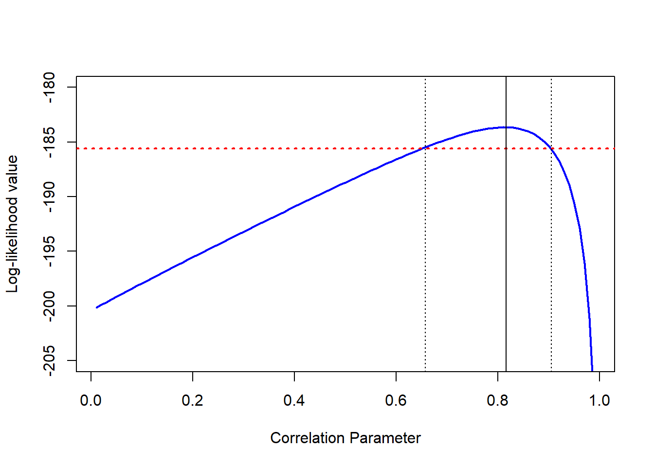
In the above plot the maximum log-likelihood value is associated with a correlation estimate of 0.816 (as given in ). The red line represents the threshold line, below which we have significant differences compared to the full (unconstrained) model. This threshold line is calculated by:
loglik.thr <- modT$loglik - chi.crit/2where is the log-likelihood value of the full model, and corresponds to the critical value for 1 df at the 5% significance level (= 3.841). Hence, any model that has a log-likelihood value smaller than -185.571 will be significantly different from our full model.
he dotted black vertical lines correspond to the places where the curve is intersected by our red threshold line. In this case, the fixed correlation values are 0.652 and 0.903, corresponding to our limits. Therefore, we can conclude that the 95% likelihood-based confidence interval for is [0.652; 0.903]. This approach provides us with a non-symmetric CI, that also restricts the parameter of interest to its natural range.
In summary, we have performed different types of statistical inference in the context of linear mixed models, particularly associated with their variance component estimates. The use of likelihood-based inferences in hypothesis testing and confidence intervals is always recommended, as it provides more accurate inferences, and it has been reported that LRT has higher power than other statistical tests. One disadvantage of this inferential approach is the need to fit several, even hundreds, of models, in contrast with the use of asymptotic distribution assumptions that only requires a single model fit.
In our full model () we have used the variance structure, but we could have used more complex and flexible variance structures, such as . For our data, this structure will have the following form:
This variance structure has extended from a single residual variance to specific variances to each of the levels of rearing. This might be a reasonable assumption, and it could be evaluated and tested using LRT by comparing these models. We leave this to the reader to explore, but this is an extension of many modelling options of linear mixed models under ASReml-R.
Author
Salvador A. Gezan
Reference
McClave, JT; Sincich, T. 2009. Statistics, 12th Edition. Prentice Hall. Upper Saddle River, NJ.
Files to download
Notes: SAG Feb-2020