ANOVA vs. linear mixed models: Choosing the right tool for your statistical analysis

Understanding ANOVA and linear mixed models (LMMs)

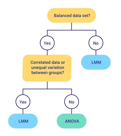
Analysis of variance (ANOVA) is a widely used statistical technique for analysing data from designed experiments. However, over recent decades, many analysts are now using linear mixed models (LMMs), also known as multi-level models, to analyse data from designed experiments instead of ANOVA. So, which method should you use?

The advantages of LMMs: Analyzing unbalanced data and modeling correlations

Like ANOVA, LMMs can analyse data with more than one source of variation, in addition to the usual residual term (e.g., data from a split-plot experiment with whole-plot and sub-plot error terms). And for balanced data sets, the LMM results are the same as those from ANOVA. However, there are several important advantages of LMMs over ANOVA. 

LMMs: Accounting for unequal variances between groups

LMMs can:

* Analyse unbalanced data sets (e.g., unbalanced designs or data sets containing missing values).

* Model correlations between observations (e.g., repeated measures data or spatial data).

* Allow for unequal variances between groups.

Genstat: A powerful tool for ANOVA and LMM analysis

Genstat has a very powerful set of ANOVA and LMM tools that are straightforward and easy to use. In Genstat, the REML algorithm is used to fit LMMs.

So why use ANOVA at all? For balanced data sets, although the LMM and ANOVA results are the same, LMM cannot provide an analysis-of-variance table. Also, the ANOVA algorithm is much more computationally efficient than the REML algorithm for fitting LMMs, so it is better to use ANOVA whenever possible.

Real-world example: Analyzing a split-plot design

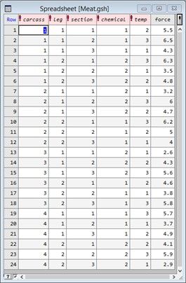
An experiment was conducted to study the effect of two meat-tenderizing chemicals and three temperatures on the force required to break strips of meat. The two hind legs were taken from four carcasses of beef and one leg was treated with chemical 1 and the other with chemical 2. Three sections were then cut from each leg and randomly allocated to three cooking temperatures. All 24 strips of meat (4 carcasses × 2 legs × 3 sections) were cooked in separate ovens. 

Notice that this experiment has a hierarchical “split-plot” design, with sections (i.e., sub-plots) nested with legs (i.e., whole-plots) nested with carcasses (i.e., blocks). The two chemicals were randomly allocated to the two legs within each carcass, and the three temperatures to the three sections within each leg.

Let’s analyse the experimental data using both ANOVA and a LMM, and compare the results. 

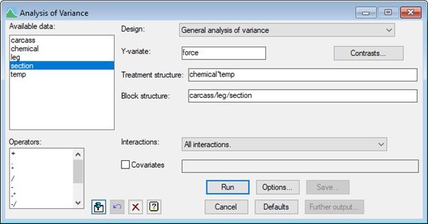
To analyse the data in Genstat using ANOVA, from the menu select Stats|Analysis of Variance|General.

The model is specified by populating the Y-variate, Treatment structure and Block structure fields as shown below.

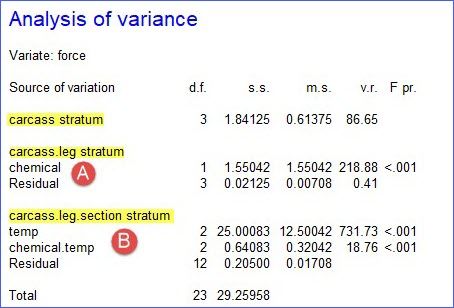
ANOVA analysis: exploring the hierarchy of strata

The ANOVA table shows that we have three strata (highlighted yellow) in the hierarchy, corresponding to the three random terms: carcass (blocks), leg within the carcass (whole-plots), and section within leg within carcass (sub-plots). The analysis automatically works out for which strata each fixed (or treatment) term is estimated and compares it with the correct residual. So, the sum of squares for the chemical is compared with a residual which represents the random variability of the legs within carcass (A). Conversely, temp and the chemical by temp interaction are compared with the residual for sections within legs (B)

.

To analyse the data using a LMM, from the menu select Stats|Mixed Models (REML)|Linear Mixed Models. The response, fixed terms and random terms in the model are specified as shown below.

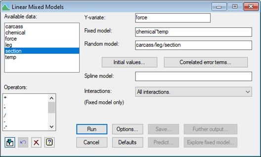
Linear mixed model analysis: Understanding variance components

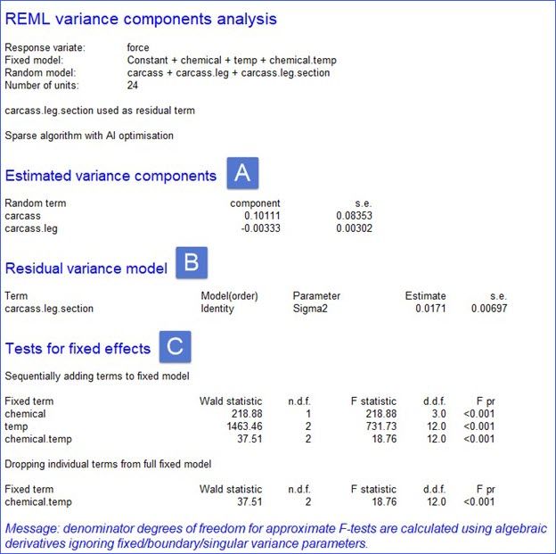
Genstat estimates a variance component for every term in the random model (A), apart from the residual. The residual (B) is a random term with a value for every unit in the design, here the 24 (4 carcasses × 2 legs × 3 sections) strips of meat. The variance component of a term measures the inherent variability of that term over and above the variability of the sub-units of which it is composed. Generally, this is positive, indicating that the units become more variable the larger they become. However, in this example the variance component for carcass.leg is negative, indicating that the legs are less variable than the sections within the legs. (This is the same conclusion we draw from the analysis of variance above by comparing the residuals in the different strata.) 

The significance of the fixed terms are assessed using F statistics (C), or, if the denominator degrees of freedom can’t be estimated, the less reliable Wald tests are used. For orthogonal (i.e., balanced) designs, the F statistics and p-values will be identical to those generated by ANOVA.  For non-orthogonal designs, the F statistics have approximate F-distributions and the order of the tests is important!

Balanced data: ANOVA's efficiency and benefit

As we have seen in the above example, for balanced data LMM and ANOVA give the same result. However, as highlighted earlier, ANOVA is preferred as it provides an analysis of variance table and the ANOVA algorithm is much more efficient than the REML algorithm used to fit the LMM.