Are breeding values (or BLUPs) a measure of risk?

Understanding BLUP-based breeding values

A BLUP-based breeding value adjusts the observed performance of a genotype according to how much information we have about that particular individual. Let’s see how this happens in more detail.

In most breeding programs phenotypic data is collected and then analyzed using linear mixed model (LMM) methodology. Wherein, genotypes are considered a random effect, and after fitting the LMM we obtain estimates of: 1) variance components, and 2) breeding values (BVs) or total genetic values (TGVs). 

Variance components are very useful they can be used to calculate heritability and therefore assess the strength of the ‘genetic’ signal of a given trait for our population. But BVs (or TGVs) are the key element, as these provide us with the deviation, or effect, of each genotype. In the case of breeding values, these correspond to the deviations that are expected from the offspring of a particular genotype when it is mated with another individual of the same genetic worth. Whereas TGVs correspond to the full genetic value of an individual (often a clone) considering both additive and non-additive effects.

As you can imagine both BV and TGV are critical in any commercial program, as they allow us to rank and then select outstanding genotypes for breeding or commercial deployment.

The role of BVs and TGVs in breeding programs

BVs and TGVs, and any other random effect from our LMM, is a BLUP effect, or best linear unbiased prediction, and this is calculated once the variance components are estimated by residual maximum likelihood. However, it is important to understand what is happening within the formulae in order to see what a BLUP really is! In order to illustrate this, we will use the following basic LMM:

where 

• is the response variable of the ith individual,
• is the breeding value of the ith individual, with , and
• is the residual/error term associated with the ith individual, with .

Here, is the additive variance, and we also have the effects all described by the numerator relationship matrix . Here, for simplicity, we will assume an identity matrix, for . Also, is the residual error variance.

Note that the above model, for simplicity, but without loss of generality, has only the overall mean in the fixed part.

Based on the above model, the expression for BLUP effects, assuming the variance-components are known (or previously estimated), is:

The full derivation is not presented here, but by following matrix algebra manipulations you can arrive to the above expression. Note here that represents the number of measurements (or copies) for the ith individual. So, for clonal values or TGVs, this corresponds to the number of copies of the same genotype. In the case of parental analysis, n will be the number of offspring from a given parent (but in this case, will be replaced by the variance associated with the General Combining ability, ).

Note that the only ‘hard’ phenotypic information about the ith genotype is its mean represented as . And the expression represents the deviation of the individual observation ‘corrected’ by all model fixed effects. In our example, the only fixed part is the overall mean.

If we had genotype as a fixed effect, and not random as above, we will be estimating the BLUE, or best linear unbiased estimation, associated with the individuals, and its expression is:

Hence, the only difference between BLUE and BLUPs is the constant: 

The shrinkage coefficient: reducing observed differences

So, what is this constant? This is often referred to as the shrinkage coefficient. This will be always less than 1, except when is infinite, or when is zero; and both of these cases are unrealistic for most breeding data.

The interesting aspect is that this coefficient will always make our observed differences (i.e., BLUEs) smaller; hence, . For example, in fruit weights let’s consider a BLUE value of 5 grams, that is the difference of a given genotype mean over the population mean; and that value might be exceptional. But if we have a shrinkage coefficient of 0.2 then this 5 grams will be reduced to 1 gram - a genetic value (or deviation) not as exciting as before!

In our shrinkage coefficient, plays an interesting role: it will reduce the magnitude of the error variance according to how much information we have. As gets larger the error term gets smaller and therefore the coefficient reaches 1. Typically, not all genotypes will have the same shrinkage coefficient, this will depend on the value of . But this is the key point of the above calculation: ‘the shrinkage of a genotype will depend on the amount of information we have about that particular genotype’. 

Let’s illustrate this with an example. Consider an analysis for a trait with a heritability of = 0.3, calculated with = 9 and = 21. Say we have a large deviation, , of 10 grams. If the replication for that genotype is small, say = 2, then its BLUP is only [9/(9 + 21/2)]x10 = 4.62. The deviation has a lot of shrinkage because there is not much ‘hard’ information on this genotype. In contrast, a genotype with the same deviation but with = 28, will have a BLUP of [9/(9 + 21/28)]x10 = 9.23 considerably less shrinkage!

Unequal shrinkage: impact on rankings and selection

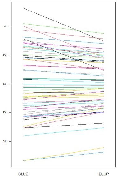
This unequal shrinkage will create important changes on the rankings between BLUEs and BLUPs, and therefore on the selection of the best individuals. This is illustrated in the spaghetti plot shown below, where the range of values is much more reduced for the BLUPs than for BLUEs.

There is another critical element to consider for the shrinkage coefficient, that is the magnitude of with respect to . If we have weak genetic control, then will be, in relative terms, much larger, and vice versa under strong genetic control. So, these variance components define the level of genetic signal in an equivalent way to the heritability . Actually, the shrinkage coefficient for = 1 is the traditional definition of heritability, and for n > 1, we have what is often known as the heritability of the mean of a genotype, or (sometimes called replicability in plant breeding).

Breeding values as a measure of risk

So, in statistical terms: what are breeding values? The answer is that they are a measure of risk, or a measure of credibility. We observe a given difference, but we do not trust it completely, so we reduce it to take into consideration its uncertainty. The interesting part is that all of this is happening internally under the mixed model framework. Hence, we will end up selecting individuals that are not only the ones with the largest differential with respect to the mean (i.e., BLUE) but also with the most credible information and therefore the least risk of been incorrect or unusual values. This is why we interpret BLUPs as a measure of risk.

The expression for the shrinkage coefficient presented above was obtained for a simple case of a LMM, but it can be easily extended to more complex models. For example, additional fixed effects can be added, and these will ‘correct’ for other differences, for example the specific block on which an individual (or experimental unit) is found. Alternatively, more complex structures for the individual, for example by adding a numerator relationship matrix , will allow us to ‘correlate’ genotype effects, and therefore, increase the replication , but in a complex way that is hard to illustrate, but often it is known as effective replication, .

There is another interesting, and linked, interpretation of the above expression for BLUP, which is associated with Bayesian statistics that combines our prior beliefs with hard evidence (i.e., data) to generate a posterior belief of the parameters of interest. But we will leave this for a future discussion.

In summary, next time you look at your estimated breeding or total genetic values from your statistical analysis remember that you are looking at values that have been adjusted by their risk of being poorly estimated; hence, you can use them with increased confidence!

About the author

Dr. Salvador Gezan is a statistician/quantitative geneticist with more than 20 years’ experience in breeding, statistical analysis and genetic improvement consulting. He currently works as a Statistical Consultant at VSN International, UK. Dr. Gezan started his career at Rothamsted Research as a biometrician, where he worked with Genstat and ASReml statistical software. Over the last 15 years he has taught ASReml workshops for companies and university researchers around the world. 

Dr. Gezan has worked on agronomy, aquaculture, forestry, entomology, medical, biological modelling, and with many commercial breeding programs, applying traditional and molecular statistical tools. His research has led to more than 100 peer reviewed publications, and he is one of the co-authors of the textbook Statistical Methods in Biology: Design and Analysis of Experiments and Regression.