The nasty politics of the average!

Often, we see reported the mean, or average, of a group of data. For example, we hear that the mean cost of a litre of regular gasoline is US $2.98. But what does this really mean? We know that the mean is a summary statistic that tells us about the data of interest, but this statistic can often be quite misleading or ‘mean’ in its interpretation!

Let’s consider another case: the monthly rainfall of approximately 50 mm (600 mm annually) for several cities in the world. Here, the cities of London (United Kingdom) and Seville (Spain) both have this precipitation, but as you might guess their patterns are very different. London has the driest month with 40 mm and wettest of 73 mm, and Seville ranges from 2 to 96 mm. That is why in London it is easier to keep the grass green! 

There are many cases like the ones above, where the mean is not sufficient to describe the process of interest properly. To illustrate some of these concepts I am going to use three different data distributions.

When average isn’t average

Before we go into more detail, let’s go back to the summary statistics. First, there are two main statistics that are commonly presented as a measure of ‘central tendency’, and a measure of ‘dispersion’. The most popular central tendencies are the mean, mode and median.

Exploring central tendencies

The mean is often represented by the arithmetic average of all available observations. The mode is the most frequent value found on the distribution of the variable, and the median is the value that is exactly at the middle of all data when they are sorted from smallest to largest. All these central tendency measures are good, but they have their specific properties.

Symmetry, skewness, and misleading statistics

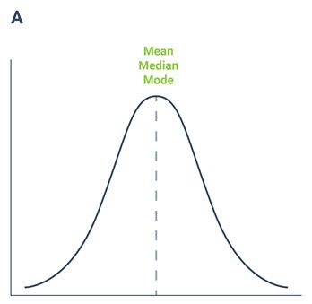
Let's consider plot A, which is a perfectly symmetrical distribution, and this, as an example, is the weight in grams of individual apples. Here we have a symmetric distribution, that resembles what is known as the ‘Normal distribution’. In this instance the mean, median and mode are almost identical with a value of 188 grams, so any could be reported. 

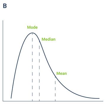
The distribution in plot B is a typical case of a skewed distribution representing, for example, the average income in a food factory. Here, there is a small group of managers with large incomes, but the majority will earn much less. For this distribution, the mean will always be larger than the median and the mode, making it a misleading statistic. In our example, the mean is US $223,000 but the median is only US $80,000 and the mode is even lower at US $38,000. Here the median is a much better representation of the centre of the data, indicating that 50% of the people earn less than $80,000 and another 50% earn more than $80,000. The arithmetic mean will be a larger, inflated value that is affected, in this case by, the salary of the CEO corresponding to two million US dollars.

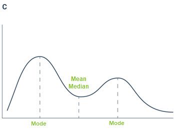
Finally, in the distribution for plot C we have the total height of a random group of students from a given college. The mean is 165.6 cm, and this value is found on the centre of the distribution. But we do have two peaks! The mode of each of these peaks is 162.3 and 174.8 cm, corresponding to the two groups we are expecting to find in this sample: females and males, respectively. In this case, we have more females in the sample than males. Here, the mean is correct, but it fails to describe the fact that we have different groups. 

Revealing variability: measures of dispersion

Hence, we see that the mean can be, and often is, a misleading ‘central tendency’ statistic. We can do better, depending on the distribution of the data, by reporting median or mode. However, this is not the full story; we also have the other group of statistics, the measures of ‘dispersion’, ‘spread’ or ‘variability’ of the data. These are also very important and provide a different angle to our data. Some of the more important measures of variability are the standard deviation, range, and percentiles.

Deviating from the truth: understanding standard deviation

The standard deviation is a complicated formula that calculates how the data is dispersed around its mean, where large values indicate more variability. Using our fictional food factory example of managers’ pay, it will be common to report that we have a mean salary of US $223,000 with a standard deviation of US $96,000. If we have a perfect Normal distribution, we often extrapolate that twice the standard deviation covers approximately 95% of the data (US $31,000 to US $415,000).

Capturing spread: the importance of range and percentiles

Often a range is more useful to describe the spread or dispersion of the data. In this same case we have a range of salaries from US $16,000 to US $2,000,000, but as you can see, this is not very informative to describe anything but the extremes; hence, we often use a range associated with percentiles. For example, we can indicate that 90% of the salaries are found between US $27,000 and US $303,000, a better description of the actual dispersion of earnings.

Mean or misleading?

As you can see, the mean is often a misleading statistic which could lead us to some incorrect interpretations, or it can provide us with incomplete pictures of the data of interest. For this reason, we always suggest to first pick the correct measure of centrality, and second, follow it with one measure of dispersion.

Nevertheless, do not forget that these are summary statistics that aim at providing you with a quick and dirty simplification of the data, and in any summarization, there will be always loss of information! So, next time you get some of these statistics think about how mean or misleading they can be!

About the author

Salvador Gezan is a statistician/quantitative geneticist with more than 20 years’ experience in breeding, statistical analysis and genetic improvement consulting. He currently works as a Statistical Consultant at VSN International, UK. Dr. Gezan started his career at Rothamsted Research as a biometrician, where he worked with Genstat and ASReml statistical software. Over the last 15 years he has taught ASReml workshops for companies and university researchers around the world. 

Dr. Gezan has worked on agronomy, aquaculture, forestry, entomology, medical, biological modelling, and with many commercial breeding programs, applying traditional and molecular statistical tools. His research has led to more than 100 peer reviewed publications, and he is one of the co-authors of the textbook Statistical Methods in Biology: Design and Analysis of Experiments and Regression.