How do you model the correlation structure of spatial data?

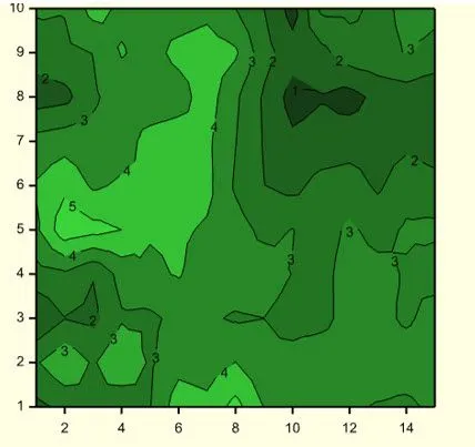
Spatial data correlation modeling: A deeper dive

In an earlier blog we discussed how to accommodate the correlation structure of repeated measures data in a linear mixed model; that is, modelling correlation in one-dimension. Now, let’s move to two-dimensions and look at modelling the correlation structure of spatial data.

So how do you measure the correlation structure of spatial data? You can use one of 4 models to measure the correlation structure of spatial data. These are Simple, Autoregressive, Power or General. Each is designed to determine a different correlation from pairs of experimental units.

Read on to find out more about how to measure the correlation structure of spatial data.   

Understanding the need for spatial correlation models

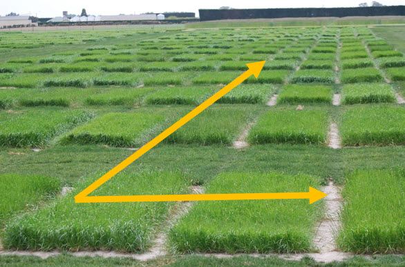
The need to model spatial correlations occurs when the experimental units are laid out in a grid, for example in a field trial or greenhouse, and where experimental units that are closer together experience more similar environmental conditions than those which are further apart. The goal of spatial modelling is to describe how the lack of independence between measurements changes as their separation in space increases or decreases.

Adequately accounting for the spatial correlation is important because it can improve the estimation of the fixed (or random) treatment effects (i.e., increases precision and reduces potential bias) by modelling more accurately the spatial distribution of the residual effects.

Visualizing an example spatial trial design

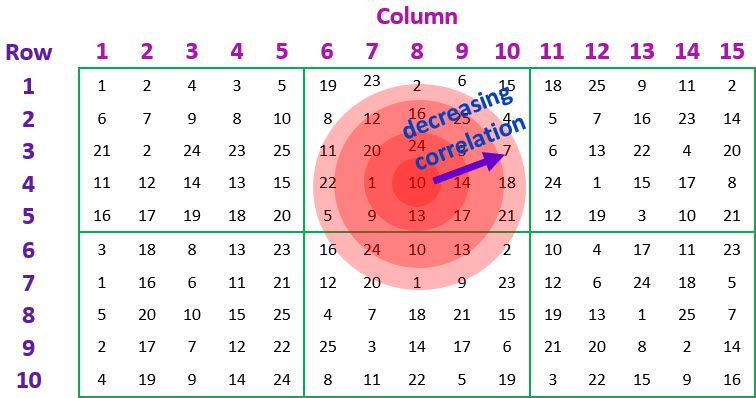
Let’s consider an example of spatial data from a field trial to compare the mean yield of 25 varieties of barley[1]. The trial design was a balanced lattice square with 6 replicates, arranged in a 15 column by 10 row regular grid of plots, as illustrated in the schematic below.

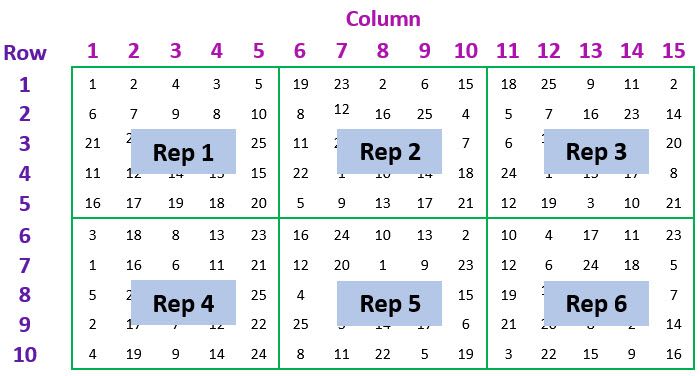
The data set contains 1 variate:

 the response variable

and 5 factors:

the replicate number (1 to 6)

the row position of the plot (i.e., experimental unit) within the trial (1 to 10)

the column position of the plot within the trial (1 to 15)

the treatment factor (1 to 25)

uniquely indexing the individual plots (i.e., has a different level for each plot in the experiment) (1 to 150)

Components of the spatial linear mixed model

The aim of the trial was to compare the mean yield of the 25 barley varieties. Thus, the response variate in the linear mixed model is , and  is the fixed term of interest.

The random model should include all terms involved in the allocation and randomization of the varieties. Failure to include these will result in the wrong denominator degrees of freedom being used to test . For this trial, the allocation of the varieties to positions (i.e., plots) in the field depended on the blocking structure of the balanced lattice design. As each replicate has a block structure of rows crossed with columns, the random model must contain  plus  within  (i.e., ) plus  within  (i.e., ).

Now let’s model the spatial correlation, which is the lack of independence between the plots (i.e., the experimental units) due to spatial proximity, meaning that nearby plots share similar microsite effects.

For the two-dimensional spatial data set, the correlation structure is fitted to the residual term - in this case defined as  by  (i.e., ), where the combination of the  and  factors represent unique positions in the spatial grid. There are many possible spatial correlation structures, but usually a separable correlation model is fitted, in which the correlation between a plot at coordinate () and a plot at coordinate () is the product of a correlation from a model defined on the rows of the experiment, and a correlation from a model defined on the columns of the experiment, i.e.

(correlation between rows apart) ×  (correlation between columns apart)

Importantly, the correlations (i.e.,  and ) are defined by correlation structures across the rows and columns of the spatial grid, respectively.

Exploring common correlation structures

Four commonly used correlation structures are described below. Note: for simplicity I’ve described them in terms of the row direction, but in all instances, you can replace row with column.

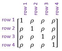
Simple correlation structure: Uniform correlation

Simple correlation structure, also known as uniform correlation. This model assumes that the correlation () between plots is constant regardless of how far apart in the row direction the plots are.

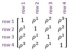
Autoregressive correlation structure: a realistic model

Autoregressive model of order 1. This model allows the correlations between plots to decrease as the distance between them in the row direction increases. This is a more realistic correlation structure for most spatial data sets than assuming constant correlation regardless of how many rows separate the plots. However, the autoregressive model should only be used when the rows are at equally spaced distances (i.e., grids with regularly spaced rows).

Power correlation structure: Flexibility for unequal spacing

Power model of order 1, also known as the city-block or exponential model. This is an alternative to the autoregressive model of order 1 which accommodates unequally spaced measurements (i.e., grids with irregularly spaced rows or columns). As with the autoregressive model, this allows the correlations between plots to decrease as the distance between them in the row direction increases.

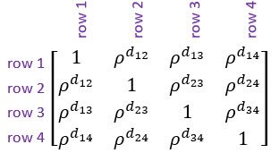
Note: is the absolute distance between the th and th rows.

General correlation structure: unstructured correlation

General correlation structure, also known as unstructured correlation. This is the most flexible correlation structure. It allows a separate correlation between every pair of rows.

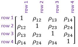
Note: is the correlation between the measurements on the th and th rows.

AR1AR1 model: Capturing spatial correlation

In most cases it is reasonable to expect the correlation between pairs of experimental units in the spatial grid to be positive, and to decrease the further apart the plots are. For a regularly spaced-grid, as in our example, such a correlation pattern can be modelled by fitting an autoregressive model of order 1 in both the row and column directions. This corresponds to what is known as an AR1AR1 separable autocorrelation model.

Adding microsite error: Incorporating variability

Finally, measurement or microsite error (also known as a nugget effect) is often needed to represent the variability, between plots, over the spatial grid correctly. That is, the data may be more variable than what can be accounted for by the spatial model alone. This additional error is allowed for by including a random term that indexes the observational units (in our data set, this term is given by ).

So, to summarize for our example:

Response variate:          

Fixed terms:                   

Random terms:             

Residual:                        

Correlation structure:   AR1AR1

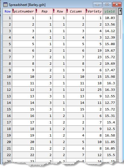
Implementing spatial correlation models in Genstat

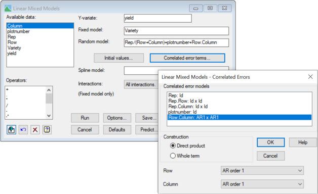
The following two screenshots show how to fit this model in Genstat, using either the:

1) Spatial Model – Regular Grid menu

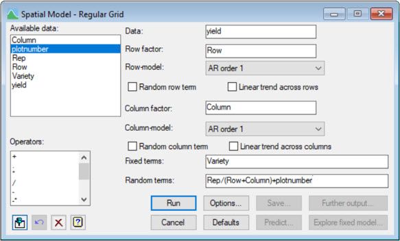
or the more general

2) Linear Mixed Models menu

As you have seen here, we can model spatial correlations between observations in two-dimensions by fitting a slightly more complex linear mixed model. Indeed, this methodology has proved particularly useful for field experiments assessing new plant varieties, where the design contains too many varieties for the conventional blocking techniques to be effective.

Correlation structure software at VSNi

At VSNi, we understand the importance of keeping our data software simple and easy to use. We have many more in-depth guides available on our website to help you become an expert on Genstat. Contact us today to enhance your spatial data research experience.

[1] Source: Gilmour, A. R., Thompson, R. and Cullis, B. R. (1995). AI, an efficient algorithm for REML estimation in linear mixed models, Biometrics51:1440-1450.

About the author

Dr. Vanessa Cave is an applied statistician interested in the application of statistics to the biosciences, in particular agriculture and ecology, and is a developer of the Genstat statistical software package. She has over 15 years of experience collaborating with scientists, using statistics to solve real-world problems.  Vanessa provides expertise on experiment and survey design, data collection and management, statistical analysis, and the interpretation of statistical findings. Her interests include statistical consultancy, mixed models, multivariate methods, statistical ecology, statistical graphics and data visualisation, and the statistical challenges related to digital agriculture.

Vanessa is currently President of the Australasian Region of the International Biometric Society, past-President of the New Zealand Statistical Association, an Associate Editor for the Agronomy Journal, on the Editorial Board of The New Zealand Veterinary Journal and an honorary academic at the University of Auckland. She has a PhD in statistics from the University of St Andrew.